Case Study: Replicating Mishra et al. (2020)

Introduction

This vignette demonstrates how to replicate the analysis from Mishra et al. (2020) of COVID-19 transmission dynamics in South Korea using EpiAwareR. This case study showcases the compositional modelling approach by building a complete epidemiological model from three reusable components.

The analysis estimates the time-varying reproduction number ( $R_t$ ) using:

AR(2) latent process for smooth evolution of log $R_t$
Renewal equation for infection dynamics
Negative binomial observation model for overdispersed case counts

Data Preparation

We use the actual South Korea COVID-19 data from the preprint, which is included in the package. The data comes from the covidregionaldata R package and contains daily confirmed cases from January to July 2020.

# Load South Korea COVID-19 data
data_path <- system.file("extdata", "south_korea_data.csv", package = "EpiAwareR")
south_korea <- read.csv(data_path)
south_korea$date <- as.Date(south_korea$date)

# Prepare full dataset - tspan will select the window
# Column must be named 'y_t' for EpiAware
full_data <- data.frame(
  date = south_korea$date,
  y_t = south_korea$cases_new
)

# Preview the training window (days 45-80)
# This corresponds to Feb 13 - Mar 19, 2020 (the main epidemic wave)
cat("Training window (tspan 45-80):\n")
#> Training window (tspan 45-80):
print(full_data[45:80, ])
#>          date y_t
#> 45 2020-02-13   0
#> 46 2020-02-14   0
#> 47 2020-02-15   0
#> 48 2020-02-16   1
#> 49 2020-02-17   1
#> 50 2020-02-18   1
#> 51 2020-02-19  15
#> 52 2020-02-20  34
#> 53 2020-02-21  75
#> 54 2020-02-22 190
#> 55 2020-02-23 256
#> 56 2020-02-24 161
#> 57 2020-02-25 130
#> 58 2020-02-26 254
#> 59 2020-02-27 449
#> 60 2020-02-28 427
#> 61 2020-02-29 909
#> 62 2020-03-01 595
#> 63 2020-03-02 686
#> 64 2020-03-03 600
#> 65 2020-03-04 516
#> 66 2020-03-05 438
#> 67 2020-03-06 518
#> 68 2020-03-07 483
#> 69 2020-03-08 367
#> 70 2020-03-09 248
#> 71 2020-03-10 131
#> 72 2020-03-11 242
#> 73 2020-03-12 114
#> 74 2020-03-13 110
#> 75 2020-03-14 107
#> 76 2020-03-15  76
#> 77 2020-03-16  74
#> 78 2020-03-17  84
#> 79 2020-03-18  93
#> 80 2020-03-19 152

# Plot the training data
plot(full_data$date[45:80], full_data$y_t[45:80], type = "b",
     xlab = "Date", ylab = "Daily Cases",
     main = "South Korea COVID-19 Cases (Feb 13 - Mar 19, 2020)")

Model Components

1. Latent Process: AR(2) Model

The AR(2) process models the evolution of log $R_t$ over time with temporal autocorrelation:

$\log R_t = \phi_1 \log R_{t-1} + \phi_2 \log R_{t-2} + \epsilon_t$

where $\epsilon_t \sim \text{Normal}(0, \sigma^2)$ .

ar2 <- AR(
  order = 2,
  damp_priors = list(
    truncnorm(0.1, 0.05, 0, 1), # ρ₁: Second-order coefficient
    truncnorm(0.8, 0.05, 0, 1)  # ρ₂: First-order (strong autocorrelation)
  ),
  init_priors = list(
    norm(-1.0, 0.1), # Initial value for lag 1
    norm(-1.0, 0.5)  # Initial value for lag 2
  ),
  std_prior = halfnorm(0.5) # σ: Innovation standard deviation
)
#> Starting Julia ...

print(ar2)
#> <EpiAware AR(2) Latent Model>
#>   Damping priors: 2 
#>   Init priors: 2 
#>   Innovation std prior: specified

Prior choices (from Mishra et al. 2020):

First-order damping coefficient ρ₂ centered at 0.8 reflects strong autocorrelation in log Rt
Second-order damping coefficient ρ₁ centered at 0.1 for smooth dynamics
Initial values centered at -1 on log scale (Rt ≈ 0.37 initially)
Innovation std of 0.5 allows flexibility in Rt changes

2. Infection Model: Renewal Equation

The renewal equation models new infections based on past infections and generation time:

$I_t = R_t \sum_{s=1}^{t} I_{t-s} \cdot g_s$

where $g_s$ is the discretized generation time distribution.

renewal <- Renewal(
  gen_distribution = gamma_dist(6.5, 0.62), # Shape and scale parameters
  initialisation_prior = norm(log(1.0), 1.0) # Prior on initial log infections (wide)
)

print(renewal)
#> <EpiAware Renewal Infection Model>
#>   Generation distribution: Gamma 
#>   Initialisation prior: specified

Key parameters:

Generation time: Mean ~6.5 days (typical for COVID-19 in early 2020)
Gamma distribution allows flexible shape
Initial infections seeded near 1 with wide prior (sd=1.0 on log scale)

3. Observation Model: Negative Binomial

Links latent infections to observed case counts with overdispersion:

$Y_t \sim \text{NegBinom}(\mu = I_t, \phi)$

where $\phi$ controls overdispersion (clustering).

# The preprint fixes cluster_factor to 0.25
# We approximate this with a tight truncated normal prior
negbin <- NegativeBinomialError(
  cluster_factor_prior = truncnorm(0.25, 0.01, 0, 1)
)

print(negbin)
#> <EpiAware Negative Binomial Observation Model>
#>   Cluster factor prior: truncated(Normal(mean, sd), lower, upper)

Parameterization:

Cluster factor = $\sqrt{1/\phi}$ (coefficient of variation)
Fixed to 0.25 (via tight prior) as in the preprint
More interpretable than directly specifying $\phi$

Compose and Fit

Create Complete Model

model <- EpiProblem(
  epi_model = renewal,
  latent_model = ar2,
  observation_model = negbin,
  tspan = c(45, 80) # Exact tspan from preprint (Feb 13 - Mar 19, 2020)
)

print(model)
#> <EpiAware Epidemiological Model>
#>   Time span: 45 to 80 
#>   Components:
#>     - Infection model: epiaware_renewal 
#>     - Latent model: epiaware_ar 
#>     - Observation model: epiaware_negbin

The EpiProblem combines components into a joint Bayesian model with automatic validation. The tspan = c(45, 80) selects days 45-80 from the full dataset, matching the preprint exactly.

Bayesian Inference

We use NUTS (No-U-Turn Sampler) with Pathfinder initialization for posterior inference:

results <- fit(
  model = model,
  data = full_data, # Pass full dataset; tspan selects the window
  method = nuts_sampler(
    warmup = 1000, # Adaptation iterations
    draws = 2000, # Posterior samples per chain (matches preprint)
    chains = 4 # Independent chains for convergence assessment
  )
)
#> Generating Turing.jl model...
#> Running NUTS sampling...
#>   Chains: 4
#>   Warmup: 1000
#>   Draws: 2000
#>   Running Pathfinder initialization...
#>   Pathfinder init failed, using default initialization...
#> Processing results...

Note: Fitting typically takes 2-5 minutes on modern hardware.

Results

Convergence Diagnostics

print(results)
#> <EpiAware Model Fit>
#> 
#> Model:
#>   Time span: 45 to 80 
#>   Infection model: epiaware_renewal 
#>   Latent model: epiaware_ar 
#>   Observation model: epiaware_negbin 
#> 
#> Sampling:
#>   Method: NUTS
#>   Chains: 4 
#>   Draws: 2000 (per chain)
#> 
#> Convergence:
#>   Max Rhat: 1.109 
#>   Min ESS (bulk): 38 
#>   Warning: Some parameters have Rhat > 1.1
#>   Warning: Some parameters have ESS < 100
#> 
#> Use summary() for parameter estimates
#> Use plot() to visualize results

Check for:

Rhat < 1.1: Chains have converged to the same distribution
ESS > 100: Sufficient effective sample size for inference
No divergent transitions: NUTS is exploring the posterior efficiently

Parameter Summaries

# Detailed posterior summaries
summary(results)
#> # A tibble: 53 × 10
#>    variable    mean  median     sd    mad      q5    q95  rhat ess_bulk ess_tail
#>    <chr>      <dbl>   <dbl>  <dbl>  <dbl>   <dbl>  <dbl> <dbl>    <dbl>    <dbl>
#>  1 latent.… -0.993  -0.991  0.0975 0.0950 -1.16   -0.833  1.00    9221.    6044.
#>  2 latent.… -0.650  -0.645  0.476  0.467  -1.44    0.121  1.00    5286.    5048.
#>  3 latent.…  0.0843  0.0833 0.0399 0.0415  0.0205  0.153  1.00    5170.    3271.
#>  4 latent.…  0.810   0.810  0.0451 0.0436  0.736   0.886  1.00     784.     178.
#>  5 latent.…  0.555   0.549  0.0882 0.0843  0.422   0.710  1.00    3136.    4360.
#>  6 latent.…  0.991   1.00   0.926  0.928  -0.546   2.50   1.00    5799.    6105.
#>  7 latent.…  1.36    1.35   0.921  0.942  -0.131   2.85   1.00    2814.    5285.
#>  8 latent.…  1.23    1.23   0.920  0.940  -0.279   2.76   1.00    7287.    5747.
#>  9 latent.…  1.18    1.16   0.878  0.879  -0.242   2.65   1.00    7113.    5672.
#> 10 latent.…  2.16    2.16   0.819  0.815   0.809   3.53   1.00    8267.    5700.
#> # ℹ 43 more rows

Key parameters to examine:

AR damping coefficients ( $\phi_1$ , $\phi_2$ ): Autocorrelation strength
Innovation std ( $\sigma$ ): Variability in $R_t$ changes
Cluster factor: Degree of case count overdispersion
Initial infections: Epidemic seeding

Working with posterior draws

epiaware_fit objects integrate directly with the posterior package. You can convert the samples to any draws format for use with bayesplot, loo, or other packages:

library(posterior)
#> This is posterior version 1.7.0
#> 
#> Attaching package: 'posterior'
#> The following objects are masked from 'package:stats':
#> 
#>     mad, sd, var
#> The following objects are masked from 'package:base':
#> 
#>     %in%, match

# Convert to draws_df for tidy workflows
draws <- as_draws_df(results)
head(draws)
#> # A draws_df: 6 iterations, 1 chains, and 53 variables
#>   latent.ar_init.1. latent.ar_init.2. latent.damp_AR.1. latent.damp_AR.2.
#> 1             -0.95             -0.14             0.090              0.74
#> 2             -0.87             -1.63             0.040              0.73
#> 3             -0.88             -0.44             0.081              0.74
#> 4             -0.94             -0.74             0.050              0.77
#> 5             -0.96             -0.86             0.082              0.75
#> 6             -0.98              0.10             0.081              0.78
#>   latent.std latent.ϵ_t.1. latent.ϵ_t.2. latent.ϵ_t.3.
#> 1       0.49          0.52          1.07         -0.99
#> 2       0.53          0.70          1.24          1.06
#> 3       0.42          0.58          2.27          0.95
#> 4       0.58          1.61          0.68          1.99
#> 5       0.54          1.72          1.18          1.76
#> 6       0.44          1.16          1.82          1.10
#> # ... with 45 more variables
#> # ... hidden reserved variables {'.chain', '.iteration', '.draw'}

# Find AR damping and std parameters by pattern
all_vars <- variables(draws)
ar_vars <- grep("damp_AR|latent\\.std", all_vars, value = TRUE)
ar_vars
#> [1] "latent.damp_AR.1." "latent.damp_AR.2." "latent.std"

# Summarise the AR-related parameters
subset_draws(draws, variable = ar_vars) |>
  summarise_draws()
#> # A tibble: 3 × 10
#>   variable        mean median     sd    mad     q5   q95  rhat ess_bulk ess_tail
#>   <chr>          <dbl>  <dbl>  <dbl>  <dbl>  <dbl> <dbl> <dbl>    <dbl>    <dbl>
#> 1 latent.damp_… 0.0843 0.0833 0.0399 0.0415 0.0205 0.153  1.00    5170.    3271.
#> 2 latent.damp_… 0.810  0.810  0.0451 0.0436 0.736  0.886  1.00     784.     178.
#> 3 latent.std    0.555  0.549  0.0882 0.0843 0.422  0.710  1.00    3136.    4360.

This also enables bayesplot diagnostics:

library(bayesplot)

# Trace plots for AR damping coefficients
damp_vars <- grep("damp_AR", variables(as_draws_array(results)), value = TRUE)
mcmc_trace(as_draws_array(results), pars = damp_vars)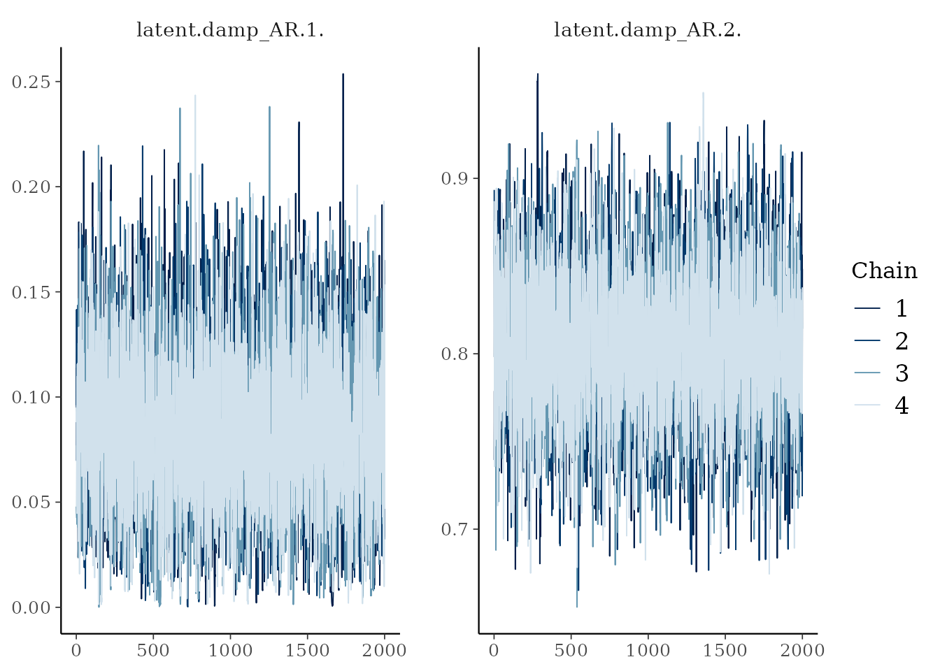

Visualization

# Time-varying reproduction number with credible intervals
plot(results, type = "Rt")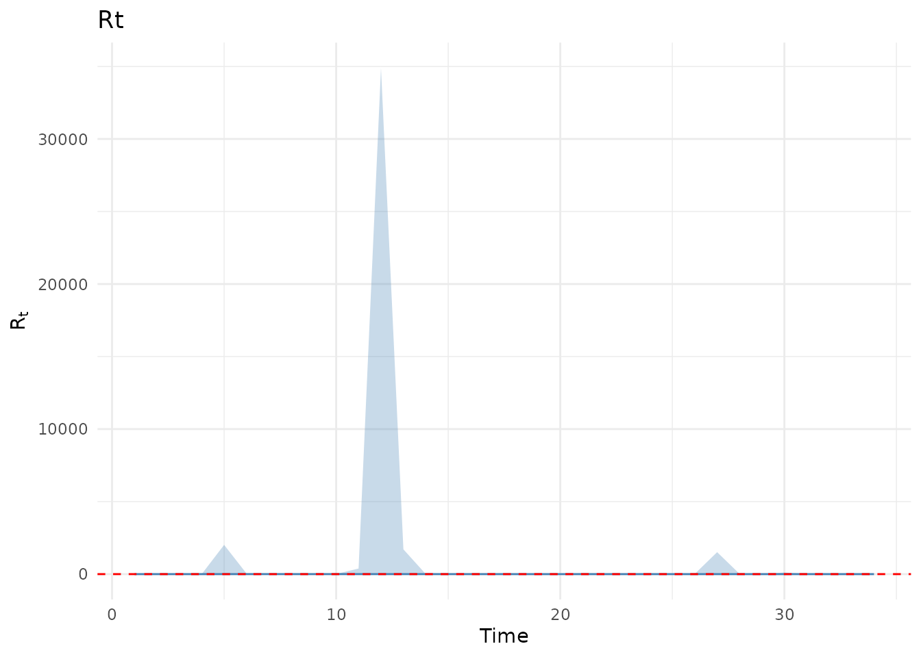


# Observed vs predicted case counts
plot(results, type = "cases")
#> Could not simulate cases from model parameters.
#> Available parameters: latent.ar_init.1., latent.ar_init.2., latent.damp_AR.1., latent.damp_AR.2., latent.std, latent.ϵ_t.1., latent.ϵ_t.2., latent.ϵ_t.3., latent.ϵ_t.4., latent.ϵ_t.5., latent.ϵ_t.6., latent.ϵ_t.7., latent.ϵ_t.8., latent.ϵ_t.9., latent.ϵ_t.10., ...


# Posterior distributions for key parameters
plot(results, type = "posterior")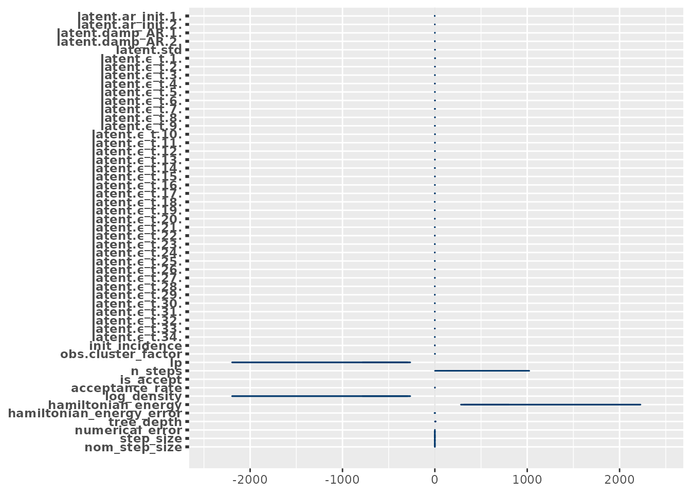

Model Comparisons

Comparing Latent Processes

Test sensitivity to AR order:

# AR(1) alternative - strong autocorrelation like AR(2)
ar1 <- AR(
  order = 1,
  damp_priors = list(truncnorm(0.8, 0.05, 0, 1)),  # High autocorrelation
  init_priors = list(norm(-1.0, 0.5)),
  std_prior = halfnorm(0.5)
)

model_ar1 <- EpiProblem(
  epi_model = renewal,
  latent_model = ar1,
  observation_model = negbin,
  tspan = c(45, 80)
)

results_ar1 <- fit(model_ar1, data = full_data)
#> Generating Turing.jl model...
#> Running NUTS sampling...
#>   Chains: 4
#>   Warmup: 1000
#>   Draws: 1000
#>   Running Pathfinder initialization...
#>   Pathfinder init failed, using default initialization...
#> Processing results...

Compare the $R_t$ estimates from both models:

library(ggplot2)
library(patchwork)

p_ar2 <- plot(results, type = "Rt") +
  ggtitle("AR(2) Model") +
  coord_cartesian(ylim = c(0, 6))

p_ar1 <- plot(results_ar1, type = "Rt") +
  ggtitle("AR(1) Model") +
  coord_cartesian(ylim = c(0, 6))

p_ar2 + p_ar1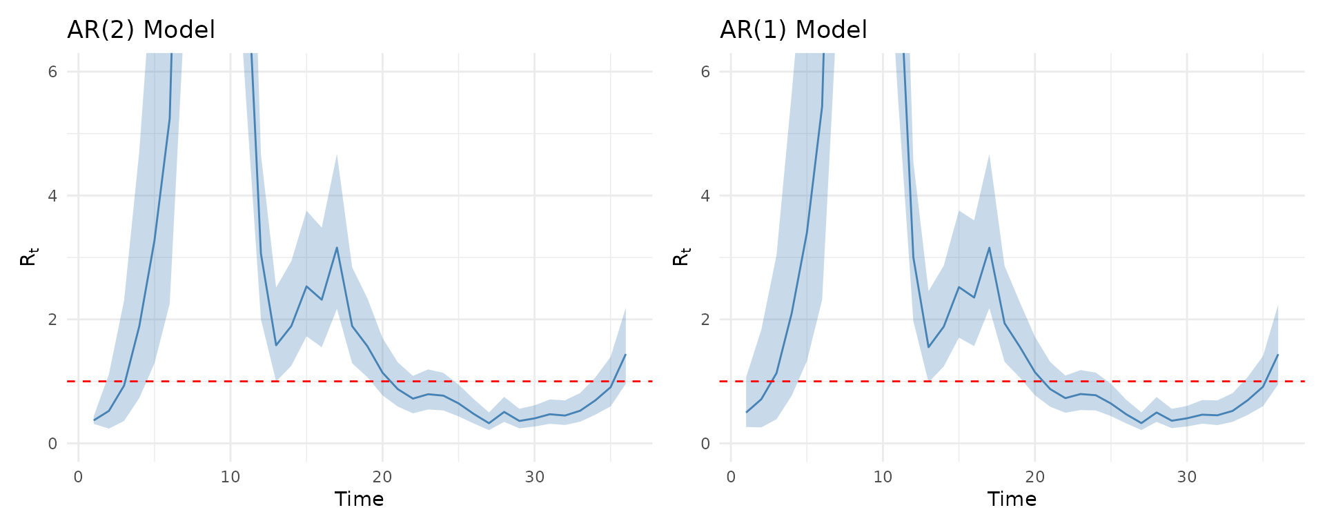

The AR(2) model typically produces smoother $R_t$ trajectories due to the additional lag term, while AR(1) may show more rapid fluctuations.

Adding Observation Delays

Account for incubation and reporting delays:

# Incubation period (~5 days)
obs_incubation <- LatentDelay(
  model = negbin,
  delay_distribution = lognorm(1.6, 0.42)
)

# Reporting delay (~2 days)
obs_full <- LatentDelay(
  model = obs_incubation,
  delay_distribution = lognorm(0.58, 0.47)
)

model_delays <- EpiProblem(
  epi_model = renewal,
  latent_model = ar2,
  observation_model = obs_full,
  tspan = c(45, 80)
)

results_delays <- fit(model_delays, data = full_data)
#> Generating Turing.jl model...
#> Running NUTS sampling...
#>   Chains: 4
#>   Warmup: 1000
#>   Draws: 1000
#>   Running Pathfinder initialization...
#>   Pathfinder init failed, using default initialization...
#> Processing results...

Compare models with and without observation delays:

p_no_delay <- plot(results, type = "Rt") +
  ggtitle("Without Delays") +
  coord_cartesian(ylim = c(0, 6))

p_delay <- plot(results_delays, type = "Rt") +
  ggtitle("With Incubation + Reporting Delays") +
  coord_cartesian(ylim = c(0, 6))

p_no_delay + p_delay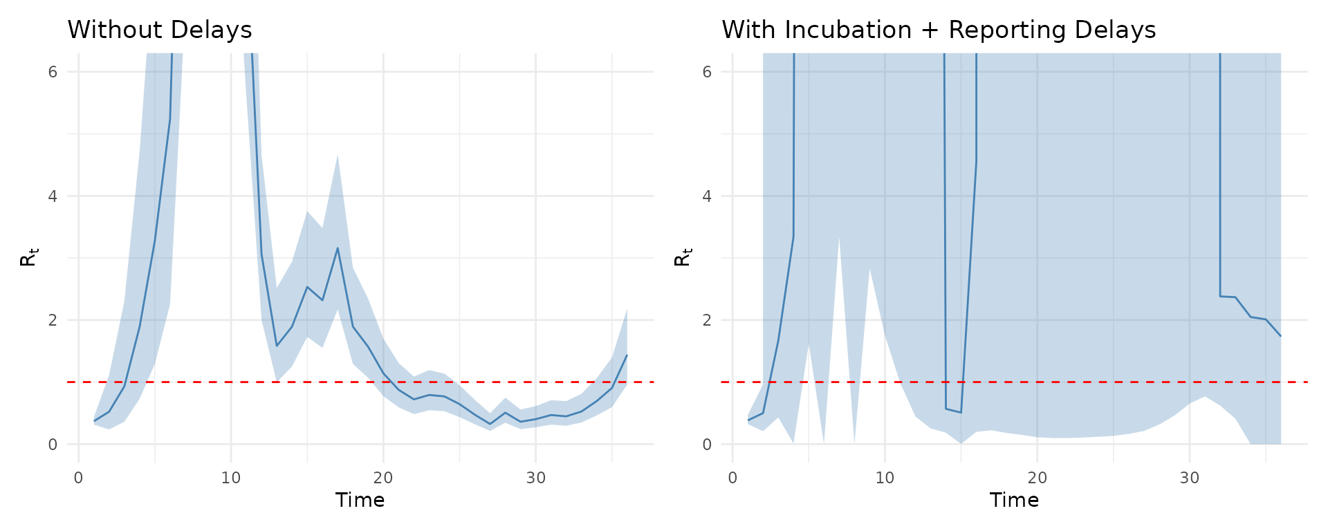

Accounting for delays shifts the $R_t$ trajectory earlier in time, as infections precede observed cases.

Interpretation

The Mishra et al. (2020) analysis demonstrated:

Flexible $R_t$ estimation: AR(2) captures both smooth trends and rapid changes
Uncertainty quantification: Bayesian credible intervals reflect parameter uncertainty
Intervention detection: Sharp decline in $R_t$ coincides with public health measures
Compositional flexibility: Easy to test alternative assumptions (AR order, delays)

Key Findings

Initial $R_t \approx 2.5$ : Rapid exponential growth phase
Post-intervention $R_t < 1$ : Control achieved through distancing measures
Moderate overdispersion: Case counts show clustering but not extreme variance
Good model fit: Posterior predictive checks show data within credible intervals

Extensions

Try modifying the analysis:

Different priors: Test sensitivity to prior choices
Alternative latent models: MA, random walk, spline models
Stratification: Separate models by age group or region
Forecast evaluation: Hold-out validation of predictive performance

References

Mishra, S., Berah, T., Mellan, T. A., et al. (2020). On the derivation of the renewal equation from an age-dependent branching process: an epidemic modelling perspective. arXiv preprint arXiv:2006.16487.

Session Info

sessionInfo()
#> R version 4.6.0 (2026-04-24)
#> Platform: x86_64-pc-linux-gnu
#> Running under: Ubuntu 24.04.4 LTS
#> 
#> Matrix products: default
#> BLAS:   /usr/lib/x86_64-linux-gnu/openblas-pthread/libblas.so.3 
#> LAPACK: /usr/lib/x86_64-linux-gnu/openblas-pthread/libopenblasp-r0.3.26.so;  LAPACK version 3.12.0
#> 
#> locale:
#>  [1] LC_CTYPE=C.UTF-8       LC_NUMERIC=C           LC_TIME=C.UTF-8       
#>  [4] LC_COLLATE=C.UTF-8     LC_MONETARY=C.UTF-8    LC_MESSAGES=C.UTF-8   
#>  [7] LC_PAPER=C.UTF-8       LC_NAME=C              LC_ADDRESS=C          
#> [10] LC_TELEPHONE=C         LC_MEASUREMENT=C.UTF-8 LC_IDENTIFICATION=C   
#> 
#> time zone: UTC
#> tzcode source: system (glibc)
#> 
#> attached base packages:
#> [1] stats     graphics  grDevices utils     datasets  methods   base     
#> 
#> other attached packages:
#> [1] patchwork_1.3.2      ggplot2_4.0.3        bayesplot_1.15.0    
#> [4] posterior_1.7.0      EpiAwareR_0.2.0.9000
#> 
#> loaded via a namespace (and not attached):
#>  [1] tensorA_0.36.2.1     sass_0.4.10          utf8_1.2.6          
#>  [4] generics_0.1.4       stringi_1.8.7        digest_0.6.39       
#>  [7] magrittr_2.0.5       evaluate_1.0.5       grid_4.6.0          
#> [10] RColorBrewer_1.1-3   fastmap_1.2.0        plyr_1.8.9          
#> [13] jsonlite_2.0.0       backports_1.5.1      scales_1.4.0        
#> [16] textshaping_1.0.5    jquerylib_0.1.4      abind_1.4-8         
#> [19] cli_3.6.6            rlang_1.2.0          withr_3.0.2         
#> [22] cachem_1.1.0         yaml_2.3.12          tools_4.6.0         
#> [25] reshape2_1.4.5       checkmate_2.3.4      JuliaConnectoR_1.1.5
#> [28] dplyr_1.2.1          vctrs_0.7.3          R6_2.6.1            
#> [31] ggridges_0.5.7       matrixStats_1.5.0    lifecycle_1.0.5     
#> [34] stringr_1.6.0        fs_2.1.0             ragg_1.5.2          
#> [37] pkgconfig_2.0.3      desc_1.4.3           pkgdown_2.2.0       
#> [40] pillar_1.11.1        bslib_0.10.0         gtable_0.3.6        
#> [43] glue_1.8.1           Rcpp_1.1.1-1.1       systemfonts_1.3.2   
#> [46] xfun_0.57            tibble_3.3.1         juliaready_0.1.0    
#> [49] tidyselect_1.2.1     knitr_1.51           farver_2.1.2        
#> [52] htmltools_0.5.9      labeling_0.4.3       rmarkdown_2.31      
#> [55] compiler_4.6.0       S7_0.2.2             distributional_0.7.0

Sebastian Funk

2026-05-05