Replicating EpiNow2 Models

Introduction

EpiNow2 is a popular R package for estimating time-varying reproduction numbers using renewal equation models. This vignette shows how to replicate a typical EpiNow2 analysis using EpiAwareR’s compositional approach.

Both packages use renewal equations and Bayesian inference, but EpiAwareR’s compositional design allows you to build a much wider class of models by assembling components.

Example: A Typical EpiNow2 Analysis

We’ll replicate a standard EpiNow2 workflow for estimating $R_t$ from case data.

Test Data

We generate simulated epidemic data with an intervention effect at day 25:

# Generate test data
set.seed(123)
dates <- seq.Date(as.Date("2024-01-01"), by = "day", length.out = 50)

# Epidemic with intervention at day 25
infections <- numeric(50)
infections[1:7] <- 30
for (i in 8:50) {
  rt <- if (i < 25) 2.0 else 0.7 # Intervention effect
  infections[i] <- rpois(1, rt * mean(infections[max(1, i - 7):(i - 1)]))
}

outbreak_data <- data.frame(
  date = dates,
  confirm = as.integer(pmax(round(infections + rnorm(50, 0, 5)), 1)) # Integer counts
)

head(outbreak_data, 10)
#>          date confirm
#> 1  2024-01-01      37
#> 2  2024-01-02      29
#> 3  2024-01-03      38
#> 4  2024-01-04      22
#> 5  2024-01-05      33
#> 6  2024-01-06      31
#> 7  2024-01-07      31
#> 8  2024-01-08      57
#> 9  2024-01-09      73
#> 10 2024-01-10      63

Step 1: The EpiNow2 Approach

First, we run EpiNow2. Note: EpiNow2 must be loaded and run before EpiAwareR due to a runtime conflict between Stan and Julia.

library(EpiNow2)

# Define generation time (mean ~5 days)
generation_time <- Gamma(
  mean = 5.0,
  sd = 2.0
)

# No reporting delay for this simple example (data is directly observed)
# For real data, you would add: delays = delay_opts(reporting_delay)

# Use daily random walk for Rt (alternative to GP)
rt_settings <- rt_opts(
  prior = Normal(mean = 1, sd = 0.5), # Tighter prior
  rw = 1 # Daily random walk
)

# Run estimation with timing
# Wrap in tryCatch to handle CI environments where Stan may fail
epinow2_results <- NULL
epinow2_time <- tryCatch({
  system.time({
    epinow2_results <- epinow(
      outbreak_data,
      generation_time = generation_time_opts(generation_time),
      rt = rt_settings,
      stan = stan_opts(cores = 2, chains = 2, samples = 500, warmup = 250)
    )
  })
}, error = function(e) {
  message("EpiNow2 fitting failed (may occur in some CI environments): ", e$message)
  NULL
})

if (!is.null(epinow2_results)) {
  cat("EpiNow2 runtime:", epinow2_time["elapsed"], "seconds\n")
  summary(epinow2_results)
  plot(epinow2_results)
} else {
  cat("EpiNow2 results not available - see message above\n")
}
#> EpiNow2 runtime: 52.568 seconds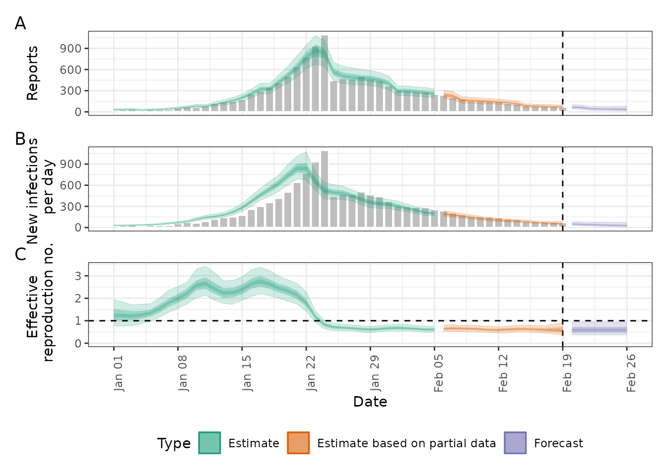

The rw = 1 option creates a daily random walk for $R_t$ , which is an alternative choice to the default Gaussian Process.

Step 2: The EpiAwareR Equivalent

Now we load EpiAwareR and replicate the analysis. We explicitly build the model from components:

library(EpiAwareR)

# 1. Latent process: daily random walk for Rt
# AR(1) with damping ≈ 1 creates a random walk (equivalent to EpiNow2's rw=1)
latent <- AR(
  order = 1,
  damp_priors = list(truncnorm(0.99, 0.01, 0.9, 1)), # Near 1 for random walk
  init_priors = list(norm(log(1.5), 0.3)), # log(Rt) centered at 1.5 for growing epidemic
  std_prior = halfnorm(0.1)
)
#> Julia version 1.11.8 at location /opt/hostedtoolcache/julia/1.11.8/x64/bin will be used.
#> Loading setup script for JuliaCall...
#> Finish loading setup script for JuliaCall.
#> EpiAware Julia backend loaded successfully

# 2. Infection model: renewal equation with generation time
# EpiNow2: Gamma(mean=5, sd=2) -> shape=6.25, scale=0.8
infection <- Renewal(
  gen_distribution = gamma_dist(6.25, 0.8),
  initialisation_prior = norm(log(30), 0.5) # Match simulated initial infections
)

# 3. Observation model: negative binomial (no delay for this simple example)
observation <- NegativeBinomialError(
  cluster_factor_prior = halfnorm(0.5)
)

# 4. Compose into complete model
model <- EpiProblem(
  epi_model = infection,
  latent_model = latent,
  observation_model = observation,
  tspan = c(1, 50)
)

print(model)
#> <EpiAware Epidemiological Model>
#>   Time span: 1 to 50 
#>   Components:
#>     - Infection model: epiaware_renewal 
#>     - Latent model: epiaware_ar 
#>     - Observation model: epiaware_negbin

Fit the Model

# Run estimation with timing (2 chains to match EpiNow2)
epiaware_time <- system.time({
  results <- fit(
    model = model,
    data = outbreak_data,
    method = nuts_sampler(
      warmup = 250,
      draws = 500,
      chains = 2
    )
  )
})
#> Generating Turing.jl model...
#> Running NUTS sampling...
#>   Chains: 2
#>   Warmup: 250
#>   Draws: 500
#>   Running Pathfinder initialization...
#>   Pathfinder initialization failed, using default initialization...
#> Processing results...

cat("EpiAwareR runtime:", epiaware_time["elapsed"], "seconds\n")
#> EpiAwareR runtime: 529.725 seconds

# View results
print(results)
#> <EpiAware Model Fit>
#> 
#> Model:
#>   Time span: 1 to 50 
#>   Infection model: epiaware_renewal 
#>   Latent model: epiaware_ar 
#>   Observation model: epiaware_negbin 
#> 
#> Sampling:
#>   Method: NUTS
#>   Chains: 2 
#>   Draws: 500 (per chain)
#> 
#> Convergence:
#>   Max Rhat: 1.093 
#>   Min ESS (bulk): 75 
#>   Warning: Some parameters have ESS < 100
#> 
#> Use summary() for parameter estimates
#> Use plot() to visualize results
summary(results)
#> # A tibble: 66 × 10
#>    variable            mean  median      sd     mad      q5   q95  rhat ess_bulk
#>    <chr>              <dbl>   <dbl>   <dbl>   <dbl>   <dbl> <dbl> <dbl>    <dbl>
#>  1 latent.ar_init.…  0.348   0.350  0.247   0.255   -0.0342 0.747 0.999     513.
#>  2 latent.damp_AR.…  0.986   0.986  0.00783 0.00810  0.971  0.997 1.01      794.
#>  3 latent.std        0.180   0.180  0.0252  0.0230   0.137  0.224 1.01      152.
#>  4 latent.ϵ_t.1.    -0.472  -0.438  0.788   0.775   -1.79   0.777 1.00      556.
#>  5 latent.ϵ_t.2.    -0.0471 -0.0754 0.771   0.748   -1.27   1.29  1.00      596.
#>  6 latent.ϵ_t.3.    -0.843  -0.838  0.786   0.774   -2.08   0.459 1.00      668.
#>  7 latent.ϵ_t.4.     0.277   0.294  0.816   0.814   -1.13   1.58  1.00      663.
#>  8 latent.ϵ_t.5.     0.0695  0.0835 0.787   0.823   -1.24   1.37  1.00      751.
#>  9 latent.ϵ_t.6.     0.476   0.472  0.770   0.758   -0.740  1.75  1.00      796.
#> 10 latent.ϵ_t.7.     1.66    1.68   0.746   0.741    0.389  2.84  1.00      616.
#> # ℹ 56 more rows
#> # ℹ 1 more variable: ess_tail <dbl>
plot(results, type = "Rt")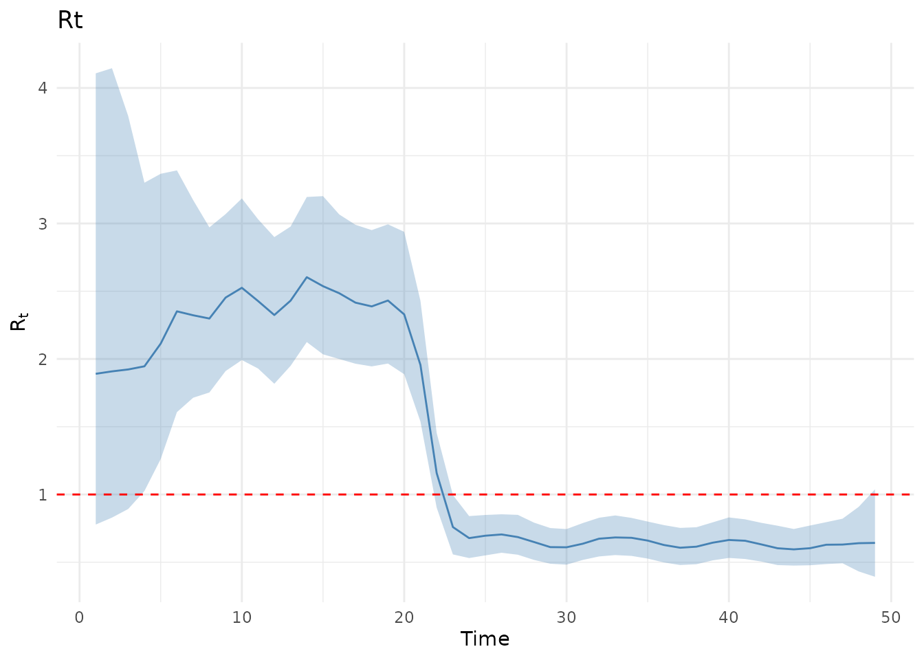

Note on initial uncertainty: Renewal models often show high uncertainty in the initial period (first ~7 days) due to limited infection history for estimating $R_t$ . This “burn-in” effect is a known characteristic of these models.

Runtime Comparison

cat("Runtime comparison (2 chains each):\n")
#> Runtime comparison (2 chains each):
if (!is.null(epinow2_time)) {
  cat("  EpiNow2:   ", round(epinow2_time["elapsed"], 1), "seconds\n")
  cat("  EpiAwareR: ", round(epiaware_time["elapsed"], 1), "seconds\n")
  cat("  Speedup:   ", round(epinow2_time["elapsed"] / epiaware_time["elapsed"], 1), "x\n")
} else {
  cat("  EpiNow2:    (not available)\n")
  cat("  EpiAwareR: ", round(epiaware_time["elapsed"], 1), "seconds\n")
}
#>   EpiNow2:    52.6 seconds
#>   EpiAwareR:  529.7 seconds
#>   Speedup:    0.1 x

Benefits of the explicit approach

EpiAwareR’s compositional design makes the model structure transparent:

Latent model explicitly states how $R_t$ evolves (random walk, AR, MA, etc.)
Infection model clearly specifies generation time and renewal dynamics
Observation model shows delays and overdispersion assumptions

This explicitness enables:

Testing alternatives: Easily compare different smoothness levels, or swap e.g. for AR(2), moving average or mechanistic models (e.g. with susceptible depletion)
Understanding priors: See exactly what distributions drive each component
Model comparison: Systematically compare competing assumptions

For example, comparing different levels of smoothness in the random walk:

# Less smooth (more variable Rt)
rw_flexible <- AR(
  order = 1,
  damp_priors = list(truncnorm(0.99, 0.01, 0.9, 1)),
  init_priors = list(norm(0, 0.5)),
  std_prior = halfnorm(0.3) # Larger innovations
)

# More smooth (less variable Rt)
rw_smooth <- AR(
  order = 1,
  damp_priors = list(truncnorm(0.99, 0.01, 0.9, 1)),
  init_priors = list(norm(0, 0.5)),
  std_prior = halfnorm(0.05) # Smaller innovations
)

# Fit both and compare
model_flexible <- EpiProblem(..., latent_model = rw_flexible, ...)
model_smooth <- EpiProblem(..., latent_model = rw_smooth, ...)

results_flexible <- fit(model_flexible, outbreak_data)
results_smooth <- fit(model_smooth, outbreak_data)

# Visual inspection of results
# Formal model comparison would require LOO cross-validation (for fit)
# or leave-future-out validation (for forecasting)
print(results_flexible)
print(results_smooth)

Learn More

EpiNow2 Documentation - The original package
Getting Started - EpiAwareR basics
Mishra Case Study - Detailed worked example

Session Info

sessionInfo()
#> R version 4.5.2 (2025-10-31)
#> Platform: x86_64-pc-linux-gnu
#> Running under: Ubuntu 24.04.3 LTS
#> 
#> Matrix products: default
#> BLAS:   /usr/lib/x86_64-linux-gnu/openblas-pthread/libblas.so.3 
#> LAPACK: /usr/lib/x86_64-linux-gnu/openblas-pthread/libopenblasp-r0.3.26.so;  LAPACK version 3.12.0
#> 
#> locale:
#>  [1] LC_CTYPE=C.UTF-8          LC_NUMERIC=C             
#>  [3] LC_TIME=C.UTF-8           LC_COLLATE=C.UTF-8       
#>  [5] LC_MONETARY=C.UTF-8       LC_MESSAGES=C.UTF-8      
#>  [7] LC_PAPER=C.UTF-8          LC_NAME=C.UTF-8          
#>  [9] LC_ADDRESS=C.UTF-8        LC_TELEPHONE=C.UTF-8     
#> [11] LC_MEASUREMENT=C.UTF-8    LC_IDENTIFICATION=C.UTF-8
#> 
#> time zone: UTC
#> tzcode source: system (glibc)
#> 
#> attached base packages:
#> [1] stats     graphics  grDevices utils     datasets  methods   base     
#> 
#> other attached packages:
#> [1] EpiAwareR_0.1.0.9000 EpiNow2_1.7.1       
#> 
#> loaded via a namespace (and not attached):
#>  [1] gtable_0.3.6          tensorA_0.36.2.1      xfun_0.56            
#>  [4] bslib_0.9.0           ggplot2_4.0.1         QuickJSR_1.9.0       
#>  [7] inline_0.3.21         vctrs_0.7.1           tools_4.5.2          
#> [10] generics_0.1.4        stats4_4.5.2          parallel_4.5.2       
#> [13] tibble_3.3.1          pkgconfig_2.0.3       R.oo_1.27.1          
#> [16] data.table_1.18.0     checkmate_2.3.3       RColorBrewer_1.1-3   
#> [19] S7_0.2.1              desc_1.4.3            distributional_0.6.0 
#> [22] RcppParallel_5.1.11-1 truncnorm_1.0-9       lifecycle_1.0.5      
#> [25] compiler_4.5.2        farver_2.1.2          textshaping_1.0.4    
#> [28] codetools_0.2-20      htmltools_0.5.9       sass_0.4.10          
#> [31] yaml_2.3.12           pillar_1.11.1         pkgdown_2.2.0        
#> [34] jquerylib_0.1.4       R.utils_2.13.0        cachem_1.1.0         
#> [37] StanHeaders_2.32.10   JuliaCall_0.17.6      abind_1.4-8          
#> [40] posterior_1.6.1       rstan_2.32.7          tidyselect_1.2.1     
#> [43] digest_0.6.39         dplyr_1.1.4           purrr_1.2.1          
#> [46] labeling_0.4.3        fastmap_1.2.0         grid_4.5.2           
#> [49] cli_3.6.5             magrittr_2.0.4        patchwork_1.3.2      
#> [52] loo_2.9.0             utf8_1.2.6            pkgbuild_1.4.8       
#> [55] withr_3.0.2           runner_0.4.5          scales_1.4.0         
#> [58] backports_1.5.0       lubridate_1.9.4       timechange_0.3.0     
#> [61] rmarkdown_2.30        lambda.r_1.2.4        matrixStats_1.5.0    
#> [64] gridExtra_2.3         futile.logger_1.4.9   ragg_1.5.0           
#> [67] R.methodsS3_1.8.2     evaluate_1.0.5        knitr_1.51           
#> [70] rstantools_2.6.0      rlang_1.1.7           futile.options_1.0.1 
#> [73] Rcpp_1.1.1            glue_1.8.0            formatR_1.14         
#> [76] jsonlite_2.0.0        R6_2.6.1              systemfonts_1.3.1    
#> [79] fs_1.6.6

Sebastian Funk

2026-01-26