Getting Started with EpiAwareR

What is EpiAwareR?

EpiAwareR is an R interface to the Julia-based EpiAware compositional infectious disease modelling framework. It enables you to build flexible epidemiological models by composing reusable components rather than writing monolithic models from scratch.

The Compositional Approach

Instead of implementing complete models, you combine three types of components:

┌─────────────────┐
│ Latent Model    │  How Rt evolves over time
│ (e.g., AR, MA)  │  (random walk, autoregressive, etc.)
└────────┬────────┘
         │
         ↓
┌─────────────────┐
│ Infection Model │  How infections are generated
│ (e.g., Renewal) │  (renewal equation, SIR, etc.)
└────────┬────────┘
         │
         ↓
┌─────────────────┐
│ Observation     │  How infections become data
│ Model (e.g., NB)│  (negative binomial, delays, etc.)
└─────────────────┘

This “LEGO-like” approach allows you to:

Build complex models from simple, well-tested pieces
Swap components to compare different assumptions
Reuse components across studies
Leverage joint Bayesian inference for uncertainty quantification

Installation

Install EpiAwareR from GitHub:

# Install devtools if needed
if (!requireNamespace("devtools", quietly = TRUE)) {
  install.packages("devtools")
}

# Install EpiAwareR
devtools::install_github("sbfnk/EpiAwareR")

Setting Up Julia

EpiAwareR uses Julia for high-performance computation. On first use:

library(EpiAwareR)

# Automatically install Julia and EpiAware (if needed)
epiaware_setup_julia()

This will:

Install Julia (if not already present)
Install required Julia packages (EpiAware, Turing, Distributions)
Configure the Julia-R bridge

Basic Workflow

1. Prepare Your Data

EpiAwareR expects a data frame with:

Case counts: Column named y_t, cases, confirm, or counts
Dates (optional): Column named date

# Example: Simulated outbreak data
set.seed(42)
dates <- seq.Date(as.Date("2024-01-01"), by = "day", length.out = 30)

# Simple epidemic curve
cases <- c(
  5, 8, 12, 18, 27, 35, 42, 48, 52, 54,
  51, 47, 43, 38, 33, 29, 25, 22, 19, 17,
  15, 13, 12, 10, 9, 8, 7, 6, 5, 5
)

outbreak_data <- data.frame(
  date = dates,
  y_t = cases
)

head(outbreak_data)
#>         date y_t
#> 1 2024-01-01   5
#> 2 2024-01-02   8
#> 3 2024-01-03  12
#> 4 2024-01-04  18
#> 5 2024-01-05  27
#> 6 2024-01-06  35

2. Define Model Components

Latent Model: How does $R_t$ change over time?

# AR(1) process: Rt depends on its previous value
ar1 <- AR(
  order = 1,
  damp_priors = list(truncnorm(0.5, 0.2, 0, 1)), # Autocorrelation
  init_priors = list(norm(0, 0.5)), # Initial log(Rt)
  std_prior = halfnorm(0.2) # Variability
)

print(ar1)
#> <EpiAware AR(1) Latent Model>
#>   Damping priors: 1 
#>   Init priors: 1 
#>   Innovation std prior: specified

Infection Model: How are infections generated?

# Renewal equation with generation time
renewal <- Renewal(
  gen_distribution = gamma_dist(5, 1), # Mean 5 days
  initialisation_prior = norm(log(10), 1)
)

print(renewal)
#> <EpiAware Renewal Infection Model>
#>   Generation distribution: Gamma 
#>   Initialisation prior: specified

Observation Model: How do infections become observed cases?

# Negative binomial accounts for overdispersion
negbin <- NegativeBinomialError(
  cluster_factor_prior = halfnorm(0.3)
)

print(negbin)
#> <EpiAware Negative Binomial Observation Model>
#>   Cluster factor prior: truncated(Normal(0, sd), 0, Inf)

3. Compose the Model

Combine components into a complete epidemiological model:

model <- EpiProblem(
  epi_model = renewal,
  latent_model = ar1,
  observation_model = negbin,
  tspan = c(1, 30) # Days 1-30
)

print(model)
#> <EpiAware Epidemiological Model>
#>   Time span: 1 to 30 
#>   Components:
#>     - Infection model: epiaware_renewal 
#>     - Latent model: epiaware_ar 
#>     - Observation model: epiaware_negbin

4. Fit to Data

Use Bayesian MCMC to estimate parameters:

results <- fit(
  model = model,
  data = outbreak_data,
  method = nuts_sampler(
    warmup = 500,
    draws = 500,
    chains = 2
  )
)
#> Generating Turing.jl model...
#> Running NUTS sampling...
#>   Chains: 2
#>   Warmup: 500
#>   Draws: 500
#> Processing results...

5. Examine Results

# Print summary
print(results)
#> <EpiAware Model Fit>
#> 
#> Model:
#>   Time span: 1 to 30 
#>   Infection model: epiaware_renewal 
#>   Latent model: epiaware_ar 
#>   Observation model: epiaware_negbin 
#> 
#> Sampling:
#>   Method: NUTS
#>   Chains: 2 
#>   Draws: 500 (per chain)
#> 
#> Convergence:
#>   Max Rhat: Inf 
#>   Min ESS (bulk): 2 
#>   Warning: Some parameters have Rhat > 1.1
#>   Warning: Some parameters have ESS < 100
#> 
#> Use summary() for parameter estimates
#> Use plot() to visualize results

# Detailed parameter estimates
summary(results)
#> # A tibble: 46 × 10
#>    variable      mean median     sd    mad      q5   q95  rhat ess_bulk ess_tail
#>    <chr>        <dbl>  <dbl>  <dbl>  <dbl>   <dbl> <dbl> <dbl>    <dbl>    <dbl>
#>  1 latent.ar_…  0.625  0.634 0.432  0.410  -0.0617 1.32   1.00     746.     559.
#>  2 latent.dam…  0.915  0.923 0.0513 0.0481  0.826  0.984  1.00     386.     578.
#>  3 latent.std   0.215  0.210 0.0473 0.0427  0.149  0.297  1.00     564.     643.
#>  4 latent.ϵ_t…  0.721  0.717 0.956  0.971  -0.852  2.29   1.01    1474.     722.
#>  5 latent.ϵ_t…  0.965  0.983 0.855  0.833  -0.483  2.38   1.00    1768.     855.
#>  6 latent.ϵ_t…  1.08   1.09  0.800  0.833  -0.271  2.37   1.00    1600.     878.
#>  7 latent.ϵ_t…  1.01   0.993 0.866  0.876  -0.447  2.40   1.00    1319.     747.
#>  8 latent.ϵ_t…  0.617  0.665 0.863  0.822  -0.756  2.04   1.00    1102.     755.
#>  9 latent.ϵ_t…  0.138  0.143 0.764  0.785  -1.10   1.34   1.00     865.     795.
#> 10 latent.ϵ_t… -0.187 -0.189 0.740  0.744  -1.45   1.04   1.00     988.     769.
#> # ℹ 36 more rows

# Visualize
plot(results, type = "Rt")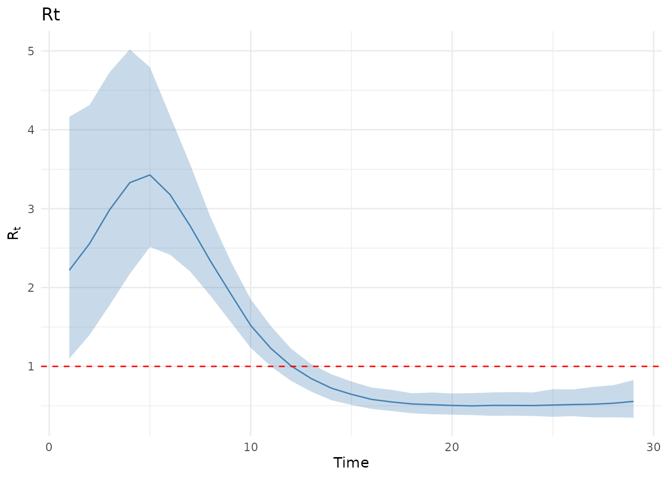

plot(results, type = "cases")
#> Posterior predictive samples not available.
#> This is a placeholder plot - full implementation would extract predictions from Julia.

Swapping Components

The power of compositional modelling: easily test different assumptions!

Different Latent Processes

# Try a random walk instead of AR(1)
rw <- AR(
  order = 1,
  damp_priors = list(truncnorm(1.0, 0.01, 0.99, 1)), # Near 1 = random walk
  init_priors = list(norm(0, 0.5)),
  std_prior = halfnorm(0.1)
)

model_rw <- EpiProblem(
  epi_model = renewal,
  latent_model = rw, # Swapped!
  observation_model = negbin,
  tspan = c(1, 30)
)

results_rw <- fit(model_rw, data = outbreak_data)

Adding Delays

# Account for reporting delay
delayed_obs <- LatentDelay(
  model = negbin,
  delay_distribution = lognorm(log(2), 0.5) # ~2 day delay
)

model_delayed <- EpiProblem(
  epi_model = renewal,
  latent_model = ar1,
  observation_model = delayed_obs, # Swapped!
  tspan = c(1, 30)
)

results_delayed <- fit(model_delayed, data = outbreak_data)

Accessing Advanced Features

For Julia features not yet wrapped in R, use epiaware_call():

# Create HierarchicalNormal error model
eps_model <- epiaware_call("HierarchicalNormal", halfnorm(0.1))

# Create MA(2) latent model
ma2 <- epiaware_call(
  "MA",
  theta_priors = list(norm(0, 0.1), norm(0, 0.1)),
  eps_t = eps_model,
  .param_map = c(theta_priors = "θ_priors", eps_t = "ϵ_t")
)

# Use in EpiProblem like any other component
model_ma <- EpiProblem(
  epi_model = renewal,
  latent_model = ma2,
  observation_model = negbin,
  tspan = c(1, 30)
)

The .param_map argument handles Greek letters in Julia parameter names.

Understanding the Components

Distribution Constructors

EpiAwareR provides convenient functions for specifying priors:

# Normal distribution
norm(mean = 0, sd = 1)

# Truncated normal (bounded)
truncnorm(mean = 0.5, sd = 0.2, lower = 0, upper = 1)

# Half-normal (positive values)
halfnorm(sd = 0.1)

# Gamma distribution
gamma_dist(shape = 5, scale = 1)

# Log-normal distribution
lognorm(meanlog = 0, sdlog = 0.5)

# Exponential distribution
exponential(rate = 0.1)

Model Classes

Each component type has specific classes:

Latent: AR(), or epiaware_call("MA", ...), etc.
Infection: Renewal(), or epiaware_call("SIR", ...), etc.
Observation: NegativeBinomialError(), LatentDelay(), etc.

Next Steps

Explore more advanced usage:

Mishra Case Study: Replicate a published analysis
EpiNow2 Comparison: Compare with EpiNow2 workflows
Model Comparison: Use LOO for model selection
Custom Models: Access cutting-edge Julia features via epiaware_call()

Getting Help

Documentation: ?AR, ?Renewal, ?fit, etc.
Issues: GitHub Issues
EpiAware Docs: Julia Documentation

Session Info

sessionInfo()
#> R version 4.5.2 (2025-10-31)
#> Platform: x86_64-pc-linux-gnu
#> Running under: Ubuntu 24.04.3 LTS
#> 
#> Matrix products: default
#> BLAS:   /usr/lib/x86_64-linux-gnu/openblas-pthread/libblas.so.3 
#> LAPACK: /usr/lib/x86_64-linux-gnu/openblas-pthread/libopenblasp-r0.3.26.so;  LAPACK version 3.12.0
#> 
#> locale:
#>  [1] LC_CTYPE=C.UTF-8          LC_NUMERIC=C             
#>  [3] LC_TIME=C.UTF-8           LC_COLLATE=C.UTF-8       
#>  [5] LC_MONETARY=C.UTF-8       LC_MESSAGES=C.UTF-8      
#>  [7] LC_PAPER=C.UTF-8          LC_NAME=C.UTF-8          
#>  [9] LC_ADDRESS=C.UTF-8        LC_TELEPHONE=C.UTF-8     
#> [11] LC_MEASUREMENT=C.UTF-8    LC_IDENTIFICATION=C.UTF-8
#> 
#> time zone: UTC
#> tzcode source: system (glibc)
#> 
#> attached base packages:
#> [1] stats     graphics  grDevices utils     datasets  methods   base     
#> 
#> other attached packages:
#> [1] EpiAwareR_0.1.0.9000
#> 
#> loaded via a namespace (and not attached):
#>  [1] gtable_0.3.6         jsonlite_2.0.0       dplyr_1.1.4         
#>  [4] compiler_4.5.2       tidyselect_1.2.1     Rcpp_1.1.0          
#>  [7] JuliaCall_0.17.6     jquerylib_0.1.4      scales_1.4.0        
#> [10] systemfonts_1.3.1    textshaping_1.0.4    yaml_2.3.12         
#> [13] fastmap_1.2.0        ggplot2_4.0.1        R6_2.6.1            
#> [16] labeling_0.4.3       generics_0.1.4       distributional_0.5.0
#> [19] knitr_1.50           backports_1.5.0      checkmate_2.3.3     
#> [22] tibble_3.3.0         desc_1.4.3           RColorBrewer_1.1-3  
#> [25] bslib_0.9.0          pillar_1.11.1        posterior_1.6.1     
#> [28] rlang_1.1.6          utf8_1.2.6           cachem_1.1.0        
#> [31] xfun_0.54            S7_0.2.1             fs_1.6.6            
#> [34] sass_0.4.10          cli_3.6.5            withr_3.0.2         
#> [37] pkgdown_2.2.0        magrittr_2.0.4       digest_0.6.39       
#> [40] grid_4.5.2           lifecycle_1.0.4      vctrs_0.6.5         
#> [43] evaluate_1.0.5       glue_1.8.0           tensorA_0.36.2.1    
#> [46] farver_2.1.2         ragg_1.5.0           abind_1.4-8         
#> [49] rmarkdown_2.30       matrixStats_1.5.0    tools_4.5.2         
#> [52] pkgconfig_2.0.3      htmltools_0.5.9

Sebastian Funk

2025-12-12