Introduction to model fitting in R
Objectives
The aim of this first session is to set you up with a framework for
model fitting. To do this, we will introduce you to the
fitR package, which we have created to facilitate
interaction during this course. This is not a full-fledged model fitting
suite. Instead, we use it to provide you with model code that follows a
common structure, as well as data and solutions to the practical
exercises.
In this session, you will
- familiarise yourselves with the structure of models in the
fitRpackage - combine the prior and likelihood to calculate the posterior for a simple SIR model
- explore the posterior of a model that has a single parameter
The first part will be mostly about introducing you to the structure we have set up – you won’t have to do much yourself in this part, but it would be worth spending some time familiarising yourself with the code and the commands, to make sure you understand what is going on. Later, you will write your own function to calculate a posterior density and use it to explore an outbreak described by a simple SIR model.
A deterministic SIR model
First, we will work with a simple deterministic SIR model. We will later fit this to a simple data set. The model has two parameters, the basic reproductive number \(R_0\) and the infectious period \(D_\mathrm{inf}\). The model equations are
\[ \begin{cases} \begin{aligned} \frac{\mathrm{d}S}{\mathrm{d}t} &= - \beta S \frac{I}{N}\\ \frac{\mathrm{d}I}{\mathrm{d}t} &= \beta S \frac{I}{N} - \nu I\\ \frac{\mathrm{d}R}{\mathrm{d}t} &= \nu I\\ \end{aligned} \end{cases} \]
where \(S\), \(I\) and \(R\) stand for the susceptible, infected and recovered compartments, respectively, \(\beta=R_0/D_\mathrm{inf}\), \(\nu = 1/D_\mathrm{inf}\) and \(N = S + I + R\) is constant. To load this model into your R session, type
data(models)This will load a few fitmodel objects into your
R session, including one called sirDeter
(for “SIR, deterministic”). A fitmodel is simply a
collection of functions and variables that define a model. Later in this
session, you might change parts of the sirDeter model. If
at any time something goes wrong, you can always go back to the original
model by typing data(models).
To see the objects that the sirDeter model contains,
type
names(sirDeter)## [1] "name" "stateNames" "thetaNames" "simulate" "rPointObs"
## [6] "dPrior" "dPointObs"A fitmodel object provides its description, as well as
the names of its state variables and parameters. These can be accessed
with
sirDeter$name## [1] "SIR with constant population size"sirDeter$stateNames## [1] "S" "I" "R"sirDeter$thetaNames## [1] "R_0" "D_inf"Moreover, each fitmodel contains four functions:
simulateto run the model,dPriorto calculate the prior density,dPointObsto calculate the log-likelihood of a given data point with respect to the model,rPointObsto generate observations from a model run.
We will now look at these one after the other. If at any time you
would like more information on the components of a
fitmodel, you can do so by typing
?fitmodelSimulate
To simulate a model run, we use the simulate command
which comes with a fitmodel (see above). To run the SIR
model, we have to provide parameter values, initial state values and the
times at which we want model output.
theta <- c(R_0 = 3, D_inf = 2)
initState <- c(S = 999, I = 1, R = 0)
times <- 1:100
traj <- sirDeter$simulate(theta, initState, times)
We can now look at the output of the model run
head(traj)## time S I R
## 1 1 999.0000 1.000000 0.0000000
## 2 2 996.4323 2.709838 0.8578584
## 3 3 989.5301 7.295046 3.1748702
## 4 4 971.3444 19.297723 9.3579062
## 5 5 925.8476 48.804024 25.3483747
## 6 6 825.2761 111.044978 63.6789335head prints the first few rows of the data set. If you
just type traj (without the head), you’ll see
the whole trajectory.
To visualise model output, you can use plotTraj.
plotTraj(traj)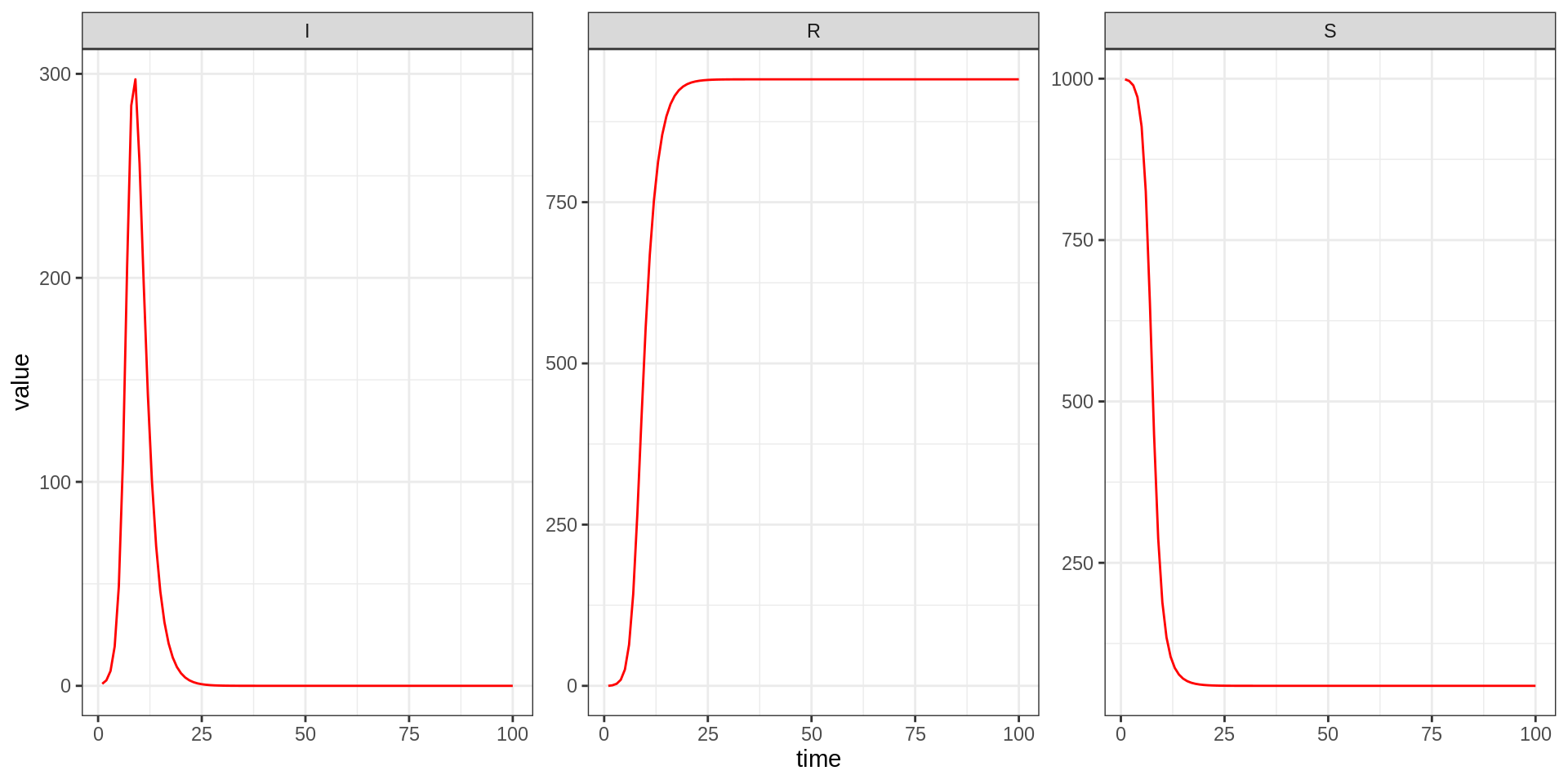
Take 10 minutes to run the model with different values of the parameters and initial state, and output times.
Remember that if you want more detail on what the functions contained
in a fitmodel do, type the function name after
sirDeter$ (or whichever fitmodel object you
are looking at; for now, we consider sirDeter). For
example, to look at the simulate function of
sirDeter, type
sirDeter$simulateThis is the key function that encodes the dynamic model we would like
to fit to data (in this case, the simple SIR model). Take 10
minutes to look at that function and let us know if you have any
questions. Tomorrow, we will give you a different
fitmodel object for a different model that comes with its
own simulate function.
Prior
To evaluate the (logarithm of the) prior for a certain combination of
parameters, use the dPrior function
sirDeter$dPrior(theta)## [1] 0.0003367003sirDeter$dPrior(theta, log = TRUE)## [1] -7.996317Have a look at the dPrior function by typing
sirDeter$dPriorYou will see that this calculates the prior of the parameters using uniform distributions on \(R_0\) (between 1 and 100) and \(D_\mathrm{inf}\) (between 0 and 30). For the moment, just have a look at it and make sure you understand it. Later, we will modify this to see how the choice of prior distributions can influence the posterior distribution.
Likelihood
The dPointObs function is used to evaluate the
likelihood of a data point. For example, the (logarithm of the)
probability density of observing a prevalence of 18 when there are 31
infectious people in the sirDeter model is
sirDeter$dPointObs(dataPoint = c(obs = 18), modelPoint = c(I = 31), theta, log = TRUE)## [1] -5.583676Have a look at the dPointObs function by typing
sirDeter$dPointObsYou will see that this calculates the likelihood of a data point
(above, an observed prevalence of 18 infections) by taking its
obs member (an observation of prevalence) and evaluating it
with respect to a Poisson distribution centred around the I
member of the model point (above, a model prevalence of 31
infections).
In other words, it assumes that the observation follows a Poisson
distribution centred around the current prevalence, and
sirDeter$dPointObs answers the question: what is the
probability of observing 18 cases when the prevalence is 31? For
the moment, just have a look at the function and make sure you
understand it. Later, we will modify this to see how the choice
of the likelihood can influence the posterior distribution.
Let’s load a test data set contained in the fitR package
using
data(epi)This contains several epidemic data sets. The first one, called
epi1, has been created using this same SIR model, with an
infectious period of 2 weeks, in a population of 1000, with 1 initial
infected and the remaining population susceptible. Later, we will try to
estimate the value of \(R_0\). You can
look at this data set using
head(epi1)## time obs
## 1 1 0
## 2 2 0
## 3 3 1
## 4 4 2
## 5 5 3
## 6 6 9The observations (“obs”) in the epi1 data set are based
on weekly observed prevalence (“I”). You can plot the data using
plotTraj(data = epi1)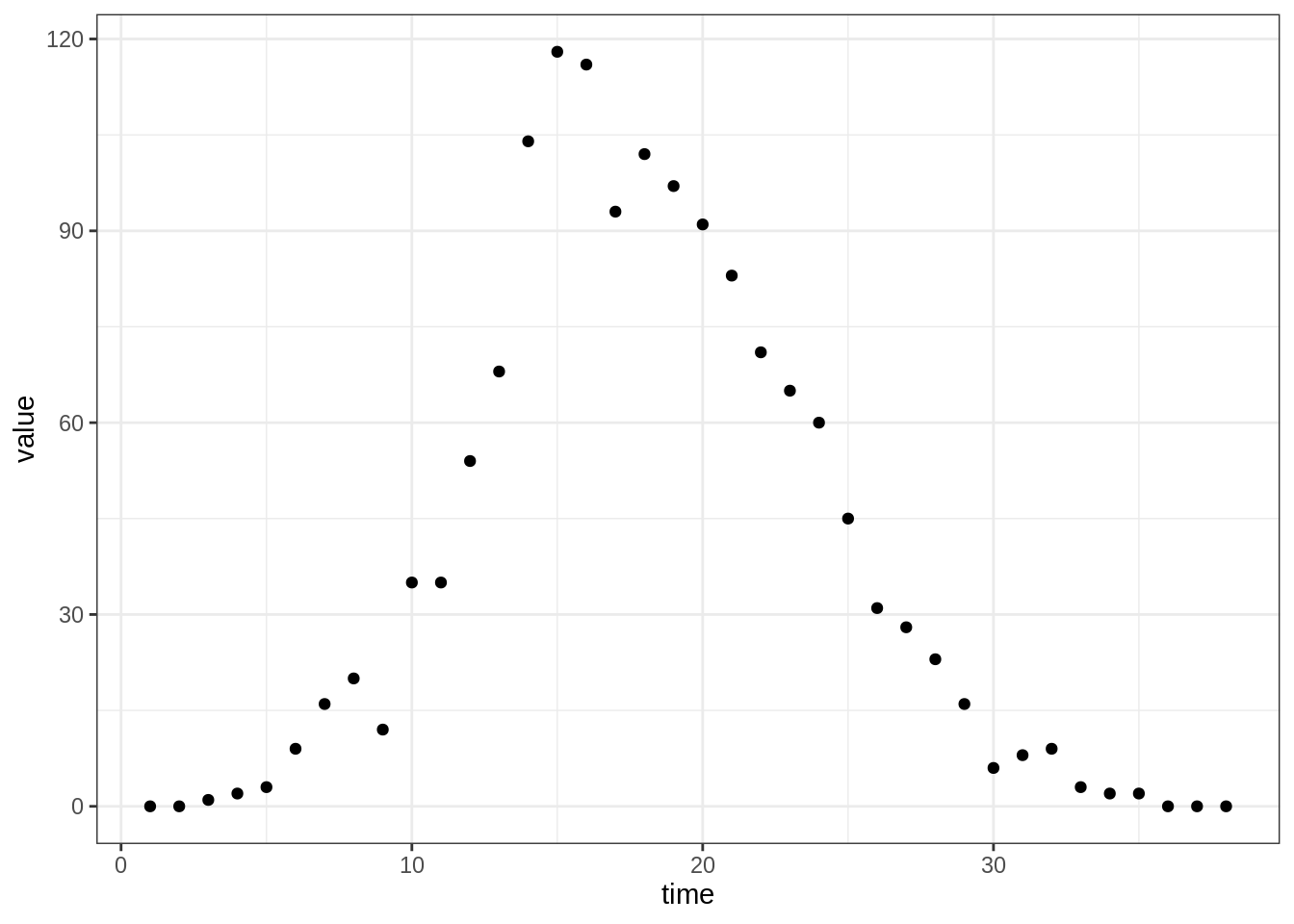
To calculate the log-likelihood of a set of parameters and initial
state, we can use the dTrajObs function contained in
fitR. This function takes a fitmodel, a
parameter vector, an initial state and a data set as arguments and
proceeds in 3 steps:
- simulate the model using the
simulatefunction of thefitmodelwith the given parameters and initial state. - evaluate the log-likelihood at every data point using the
dPointObsfunction of the model. - return the sum all the log-likelihood values.
The value returned is \(\log(p(\mathrm{Data}|X_0, \theta))\): the log-likelihood of the chosen set of parameters and initial state.
dTrajObs(sirDeter, theta, initState, epi1, log = TRUE)## [1] -3507.914Of course, you might get a different number here if you played with
the parameters. You will later need the dTrajObs function
to calculate the posterior density as a function of the parameters. Feel
free to have a look at the dTrajObs function (by typing
dTrajObs and hitting return), to see how it performs its
task.
Generate observations
The function rPointObs generates a single random
observation from a single point in a model trajectory. At the moment, we
won’t need this, but it will be later useful when it comes to model
assessment.
rPointObs can be seen as the inverse of
dPointObs. Whereas dPointObs evaluates the
likelihood at a data point with respect to the model,
rPointObs takes the model and generates a (randomly
sampled) data point.
Note also that rPointObs differs from
simulate. While simulate simulates the (in
this case, deterministic) model trajectory, rPointObs
encodes the uncertainty involved in observations to produce a random
observation point on the basis of a state of the model. To generate a
randomly observed prevalence on the basis of a true prevalence of 31, we
can write
sirDeter$rPointObs(modelPoint = c(I = 31), theta)## obs
## 24Of course, you might see a different number, as the result of this command is the outcome of a random draw.
To generate a whole trajectory with simulated observation, we have
implemented a function called rTrajObs, which can be seen
as the inverse of dTrajObs. The rTrajObs
function takes a fitmodel, a parameter vector, an initial
state and a vector of observation times as arguments and proceeds in 3
steps:
- simulate the model using the
simulatefunction of thefitmodel(see above, where you looked atsirDeter$simulate). - apply the
rPointObsfunction at every time point to generate the observations. - return the simulated trajectory, with an added column for the observations.
obsTraj <- rTrajObs(sirDeter, theta, initState, epi1$time)
head(obsTraj)
## time S I R obs
## 1 1 999.0000 1.000000 0.0000000 1
## 2 2 996.4323 2.709838 0.8578584 4
## 3 3 989.5301 7.295046 3.1748702 8
## 4 4 971.3444 19.297723 9.3579062 8
## 5 5 925.8476 48.804024 25.3483747 49
## 6 6 825.2761 111.044978 63.6789335 112If you run this multiple times, you will find that the “obs” column
is different every time. This is because the observations are results of
random draws from the (deterministic) model trajectory. If we changed
rPointObs to be deterministic (instead of a random draw
from a Poisson distribution), the outcome of rTrajObs would
be the same every time. Again, feel free to have a look at the
rTrajObs function (by simply typing rTrajObs
and hitting return), to see how it performs its task. It will be a good
idea to look at the functions that we have provided you throughout the
course.
Now you have completed the overview of a fitmodel
object, you are going use some parts of it to code a function that will
evaluate the posterior.
Calculate the posterior
Code it yourself: Write a function to calculate the value of the posterior \(p(\theta, X_0|\mathrm{Data})\) (up to a normalisation constant) for a given set of parameters and initial state, with respect to a data set.
Below you will find the skeleton of such a function. We have inserted comments for every line that you should insert. If you are struggling at any point, click on the link below the code for a more guided example.
# This is a function that takes 4 arguments:
# - fitmodel, a fitmodel object that defines the model dynamics, prior and likelihoods.
# - theta, a named vector of parameters
# - initState, a named vector of initial states
# - data, the data set we are fitting the model to
# It should return the posterior for the given model, parameters, initial state and data.
my_dLogPosterior <- function(fitmodel, theta, initState, data) {

    # calculate the `fitmodel` log-prior for parameter `theta`

    # calculate the `fitmodel` log-likelihood for parameter `theta` and
    # initial state `initState`, with respect to the data set `data`.

    # return the logged posterior probability
}
If you have trouble filling any of the empty bits in, have a look at our more guided example.
Once you are done with this, check that your function returns a sensible value.
my_dLogPosterior(sirDeter, theta, initState, epi1)## [1] -3515.91Would you expect to see the same value?
Assess the model fit
You can visually assess a model run against data using the
plotFit function, which generates an observation trajectory
from a model, parameters and initial state using rTrajObs
(see above) and plots it (lines) against the data (points).
Note that you can also simulate multiple replicates (using the
nReplicates argument) or plot the deterministic model
trajectories (using allVars = TRUE). See
?plotFit for all available options.
plotFit(sirDeter, theta, initState, epi1)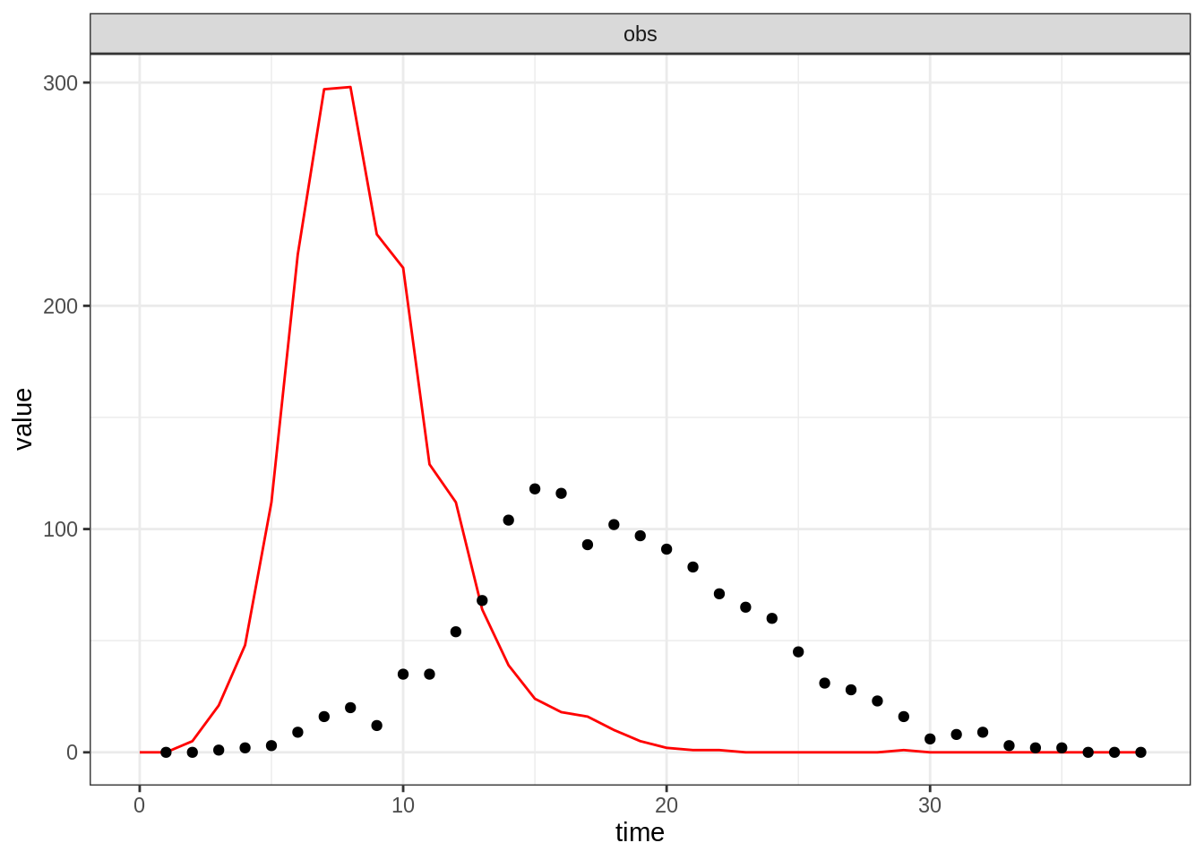
Clearly, not a very good fit on this occasion. In the next section,
you will explore the posterior distribution to find a better one.
Before that, take 10 minutes to visually assess the fit of your
model under different parameter sets and get familiar with the function
plotFit.
Explore the posterior
You are now ready to do parameter estimation by exploring the posterior at different values of the parameter. In the next practical, we will see how to automate this step using MCMC, but for now let us simply evaluate the posterior at different values of the single unknown parameter, \(R_0\).
As stated above, the infectious period of the epi1 data
set was 2 weeks. You can evaluate the posterior at different values of
\(R_0\) using the function
my_dLogPosterior you wrote above (or the one provided by
clicking through to our solution).
Take 10 minutes to figure out in which range of \(R_0\) the posterior is maximised. Does the
model fit the data (looking at plotFit)?
You can also change the prior and likelihood definitions of the
sirDeter model. Remember that you can see the definition of
sirDeter$dPrior and sirDeter$dPointObs by
typing
sirDeter$dPrior
sirDeter$dPointObs
To change the prior and likelihood functions, copy and paste the functions, change them, and reassign them to their variables. For example, to change the point log-likelihood to follow a normal distribution, you could type
sirDeter$dPointObs <- function(dataPoint, modelPoint, theta, log = FALSE) {
    # the prevalence is observed through a normally distributed process
    return(dnorm(x = dataPoint[["obs"]], mean = modelPoint[["I"]], log = log))
}
Take 20 minutes to try different distributions for the prior
and likelihood distributions (you could try, for example, to
make the prior narrower, or to use a normal distribution for the prior
using dnorm; or you could use another distribution for the
likelihood). Does the choice of distribution change the shape of
the posterior distribution?
Going further
Imperfect reporting of cases
If you knew that on average only 10% of cases were reported, how
would you change the point likelihood? You can test this with a second
data set, epi2, which you can have a look at with
head(epi2)## time obs
## 1 1 0
## 2 2 0
## 3 3 1
## 4 4 2
## 5 5 3
## 6 6 9This was created with an infectious period 2 and a reporting rate of 10%. Can you estimate \(R_0\)?
Including demographic processes and seasonal forcing
Recurrent diseases like Influenza require additional mechanisms to
explain their long-term
dynamics. To get a better feel for the code used to simulate the
model, you could modify the sirDeter model to include
demographic processes (birth & deaths) as well as a seasonal forcing
on the transmission rate of the pathogen (several solutions are
possible).
This web site and the material contained in it were originally created in support of an annual short course on Model Fitting and Inference for Infectious Disease Dynamics at the London School of Hygiene & Tropical Medicine. All material is under a MIT license. Please report any issues or suggestions for improvement on the corresponding GitHub issue tracker. We are always keen to hear about any uses of the material here, so please do get in touch using the Discussion board if you have any questions or ideas, or if you find the material here useful or use it in your own teaching.