Putting it all together

Stochastic models and the state-space view

The state-space view

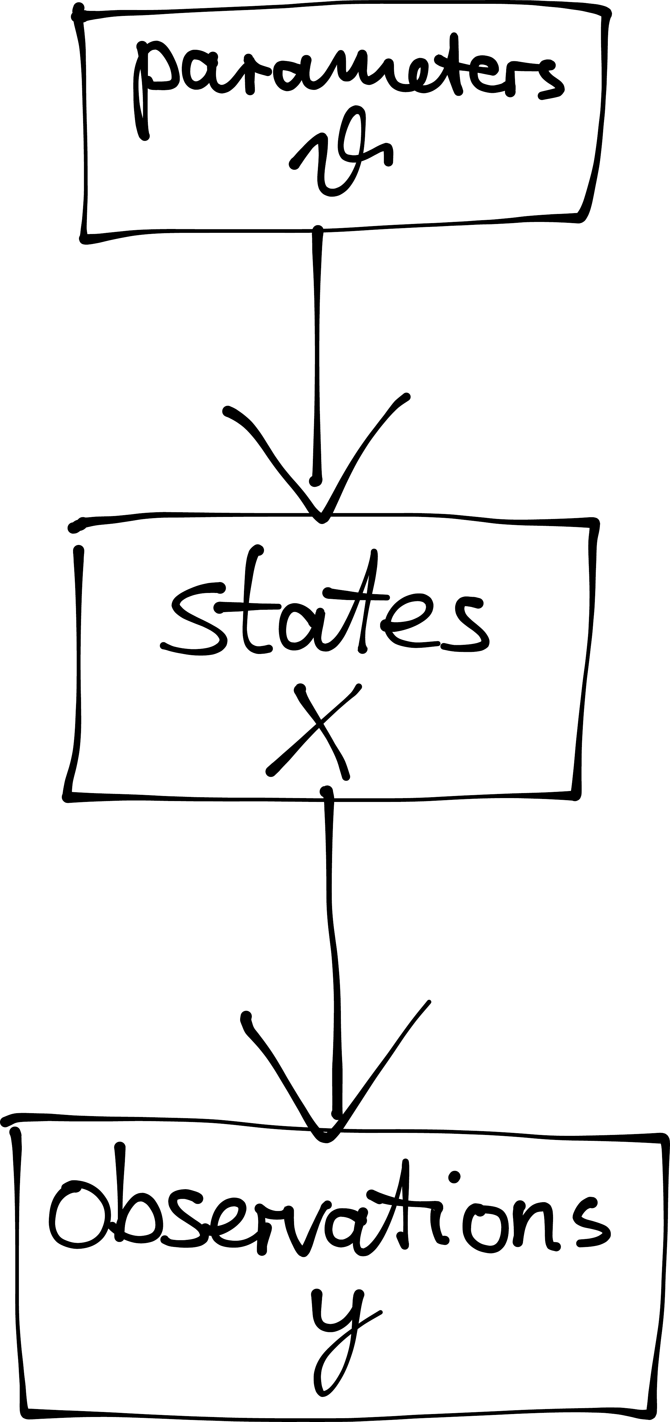
What we really want to know

We want to find out two things:

  1. the parameters of the process, \(\theta\)
  2. the state process, \(x\), as opposed to what we observe

We want to do this on the basis of observations (data), \(y\).

Hierarchical model

This kind of model is sometimes called a Bayesian hierarchical model.

Example: influenza in the UK
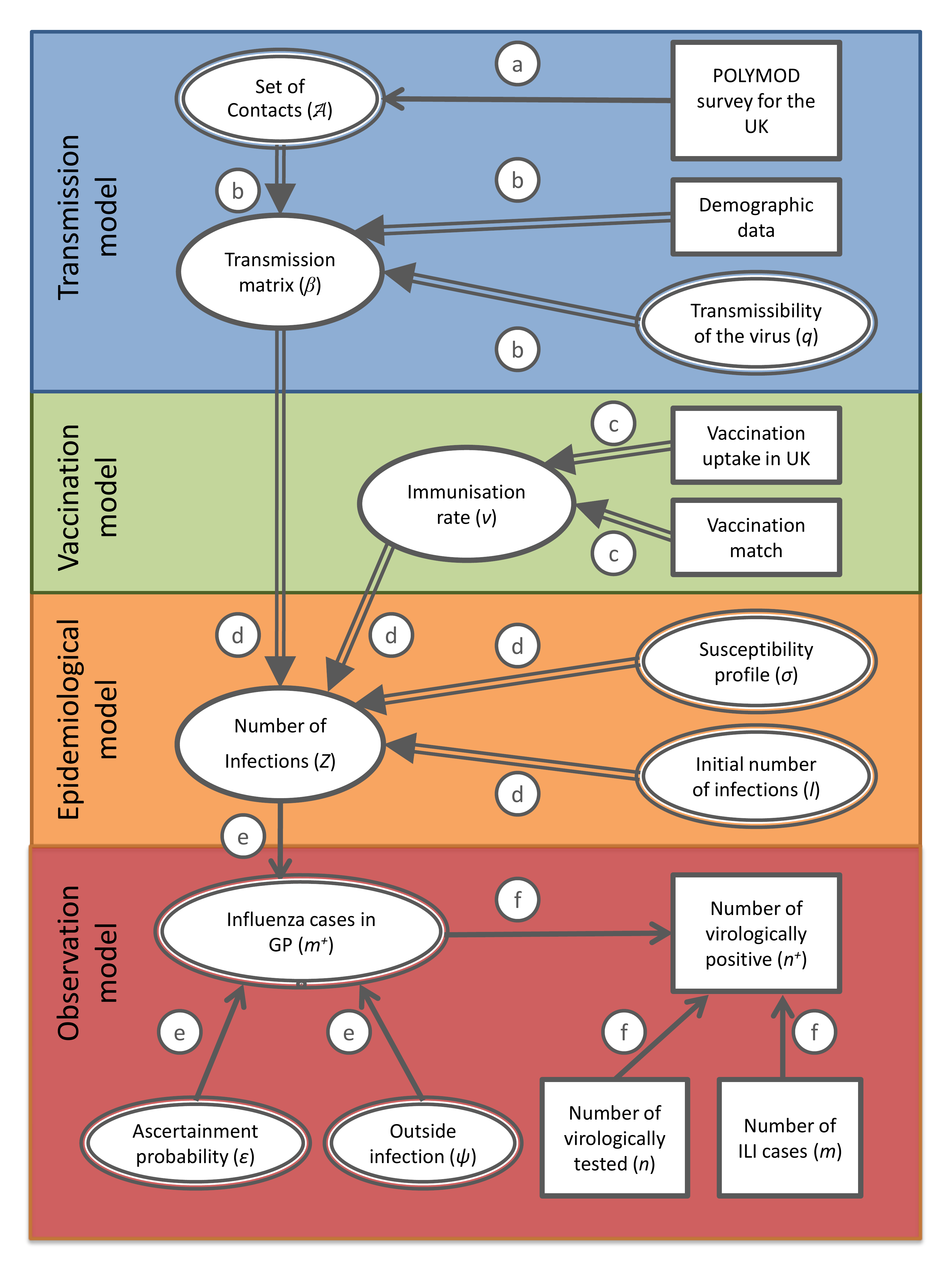
Baguelin et al. (2013)

Combining the probabilities

  1. prior probabilities of the parameters \[p(\theta)\]
  2. model trajectories \[p(x \mid \theta)\]
  3. observations \[p(y \mid x, \theta)\]

Applying the chain rule gives the joint probability

\[p(y, x, \theta) = p(y \mid x, \theta)\, p(x \mid \theta)\, p(\theta)\]
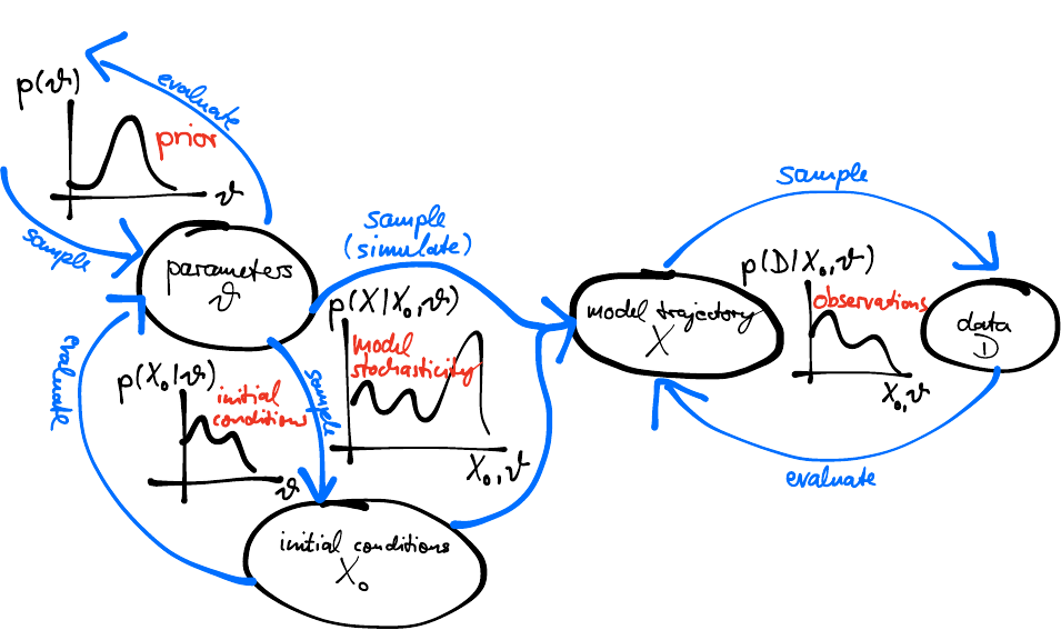
Fitting a state-space model

Doing inference

The joint probability

\[p(y, x, \theta) = p(y \mid x, \theta)\, p(x \mid \theta)\, p(\theta)\]

encodes everything about our model.

To do model fitting and inference, set \(y\) to the data we observe and calculate the posterior

\[p(x, \theta \mid y) = \frac{p(y, x, \theta)}{p(y)}\]

We can rewrite this as

\[p(x, \theta \mid y) = p(\theta \mid y)\, p(x \mid \theta, y)\]

  • the first factor is what we need for parameter fitting
  • the second factor is what we need for state estimation

Parameter estimation

\[p(x, \theta \mid y) = p(\theta \mid y)\, p(x \mid \theta, y)\]

  • In a deterministic model, every \(\theta\) leads to one possible \(x_{\theta}\). In that case

    \[p(x_{\theta}, \theta \mid y) = p(\theta \mid y)\]

  • In general we cannot write down a formula for \(p(x_{\theta}, \theta, y)\). But we can sample from it.

The model we will fit

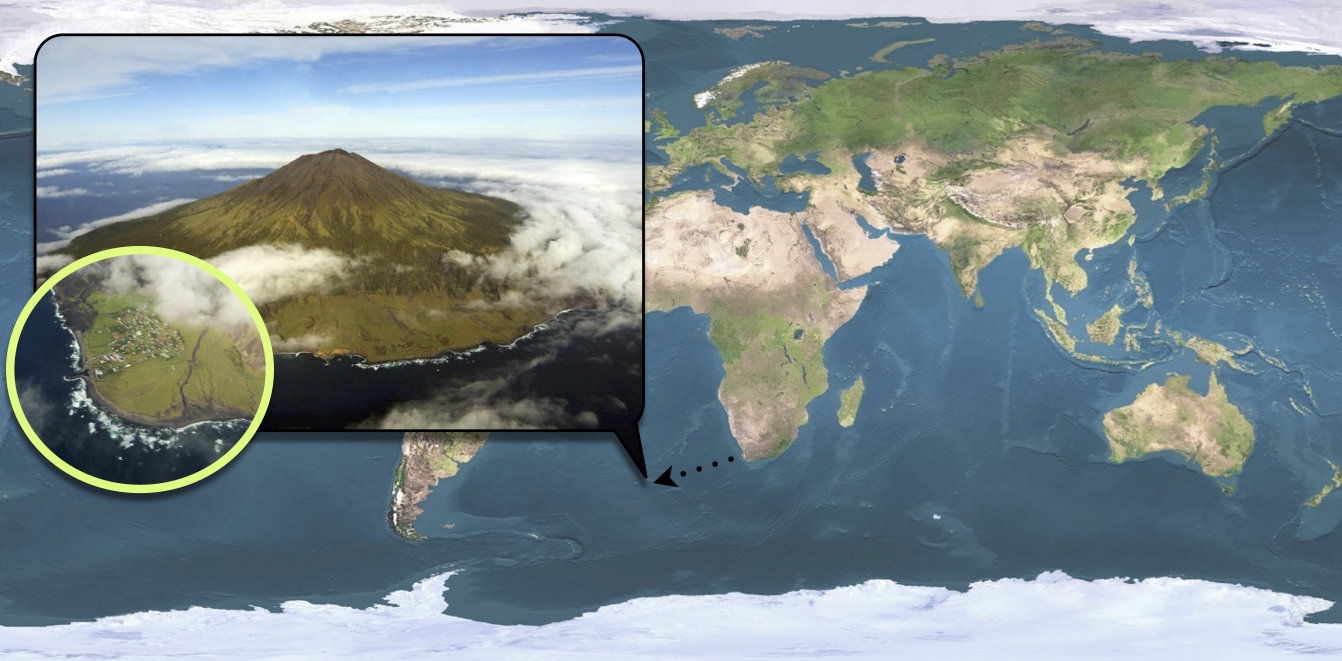
Tristan da Cunha, 1971

The most remote inhabited island in the world: 284 people, one ship every few months.

An outbreak in a closed population

An influenza-like illness arrived with a visiting ship and infected most of the island over eight weeks.

Two features make it the standard teaching example:

  • Closed — nobody arrived or left, so there is no importation to explain anything away
  • Two waves — the epidemic subsided and then came back, in a population with no new susceptibles

That second wave is the whole problem. A simple SIR model cannot produce it.

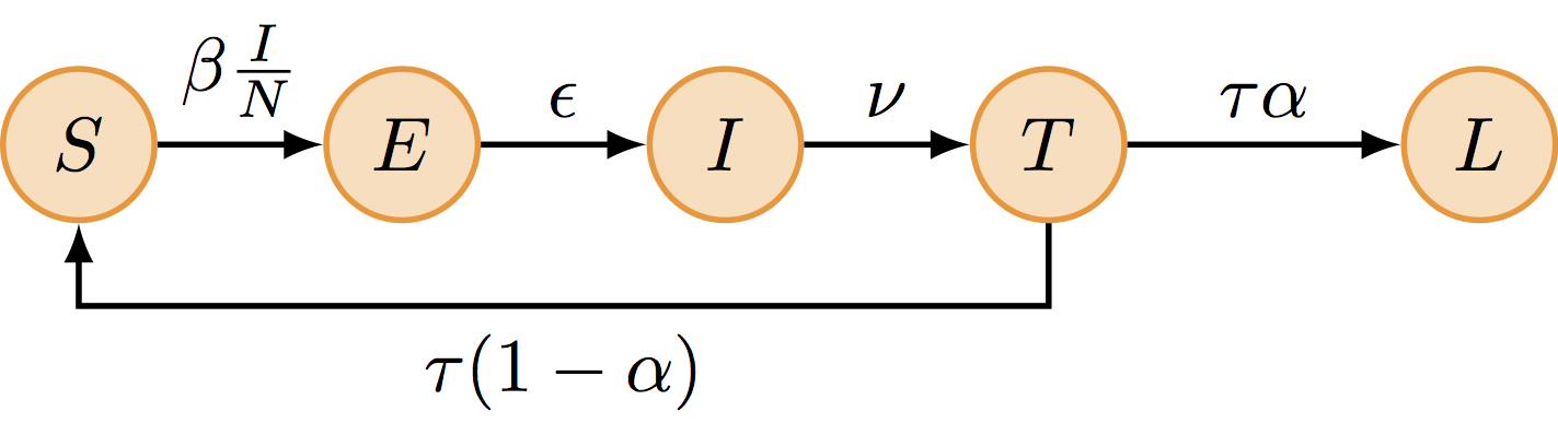
SEITL

T is temporary immunity, and only a fraction \(\alpha\) goes on to L, long-term immunity. The rest return to susceptible — and can drive a second wave.

Two independent choices

Model structure — how many compartments, and what flows between them.

Deterministic or stochastic — whether transitions are continuous flows or discrete random events.

These are separate decisions. You can simulate SEITL either way, and the practical does both so you can see the difference.

Why stochastic, here

With 284 people, chance is not a rounding error.

  • Individual runs peak days apart
  • Some fade out entirely; the deterministic model never does
  • The deterministic trajectory is not the average of the stochastic ones

Demographic noise scales roughly as \(1/\sqrt{N}\). On an island of 284 it is a first-order effect, and it is why the rest of the course needs heavier machinery.

Simulating it: Gillespie

The deterministic version solves an ODE. The stochastic version simulates events one at a time.

  1. Given the current state, compute the rate of every possible transition
  2. Draw the time to the next event from an exponential distribution
  3. Pick which event happens, with probability proportional to its rate
  4. Update the state, and repeat

Exact, and slow. Every infection and recovery is an individual event.

SEIT4L: why four compartments

A single T compartment means the waiting time in it is exponential, so the most likely thing is to leave immediately.

That is a strange claim about immunity.

Chaining four compartments, each at four times the rate, gives an Erlang waiting time: same mean, but a peak away from zero. Most people stay immune for roughly the average duration.

Your Turn

In the practical you will

  • meet the Tristan da Cunha influenza outbreak
  • build the SEITL model, which adds a latent state to the SIR structure
  • simulate it both deterministically and stochastically
  • see why the stochastic version needs different inference machinery

Return to the session