Observation models and Approximate Bayesian Computation
Model fitting and inference for infectious disease dynamics
Observation models
The choice we have been making silently
Every likelihood in this course so far has assumed
\[y_t \sim \text{Poisson}(\lambda_t)\]
where \(\lambda_t\) is what the model predicts at time \(t\).
That is a modelling choice, not a law. It encodes a specific claim about how observation works, and it has consequences.
What Poisson assumes
- The variance equals the mean. Expect 100 cases, expect a spread of about \(\pm 10\).
- Observations at different times are conditionally independent given the trajectory.
- Every case is reported independently with the same probability.
Real surveillance data rarely obliges. Weekend effects, reporting delays, outbreak investigations and clustered transmission all break these assumptions.
Overdispersion
When the data are more variable than Poisson allows, the fix is an observation model with a free variance:
\[y_t \sim \text{NegativeBinomial}(\lambda_t, \phi)\]
- \(\phi \to \infty\) recovers the Poisson
- small \(\phi\) allows a much wider spread at the same mean
The cost is one extra parameter. The benefit is that the model stops treating every unusual week as strong evidence against the trajectory.
Why it matters for inference
An observation model that is too tight makes the posterior too confident, and makes outliers dominate the fit.
A single week with 35 cases where the model expects 5 is near-impossible under Poisson, so the likelihood collapses and the sampler is dragged towards parameters that accommodate the outlier.
Under a negative binomial the same week is merely unusual.
Likelihood as a distance
Look at the negative log-likelihood of one observation as a function of how far it sits from the prediction.
That is a distance function: it scores how far the data are from the model, and different observation models are different distance functions.
- Poisson penalises large relative deviations very sharply
- Negative binomial is more forgiving in the tails
- Gaussian penalises absolute deviations symmetrically
Once you see the likelihood as a distance, an obvious question follows: what if we chose the distance directly?
Approximate Bayesian Computation
Motivation
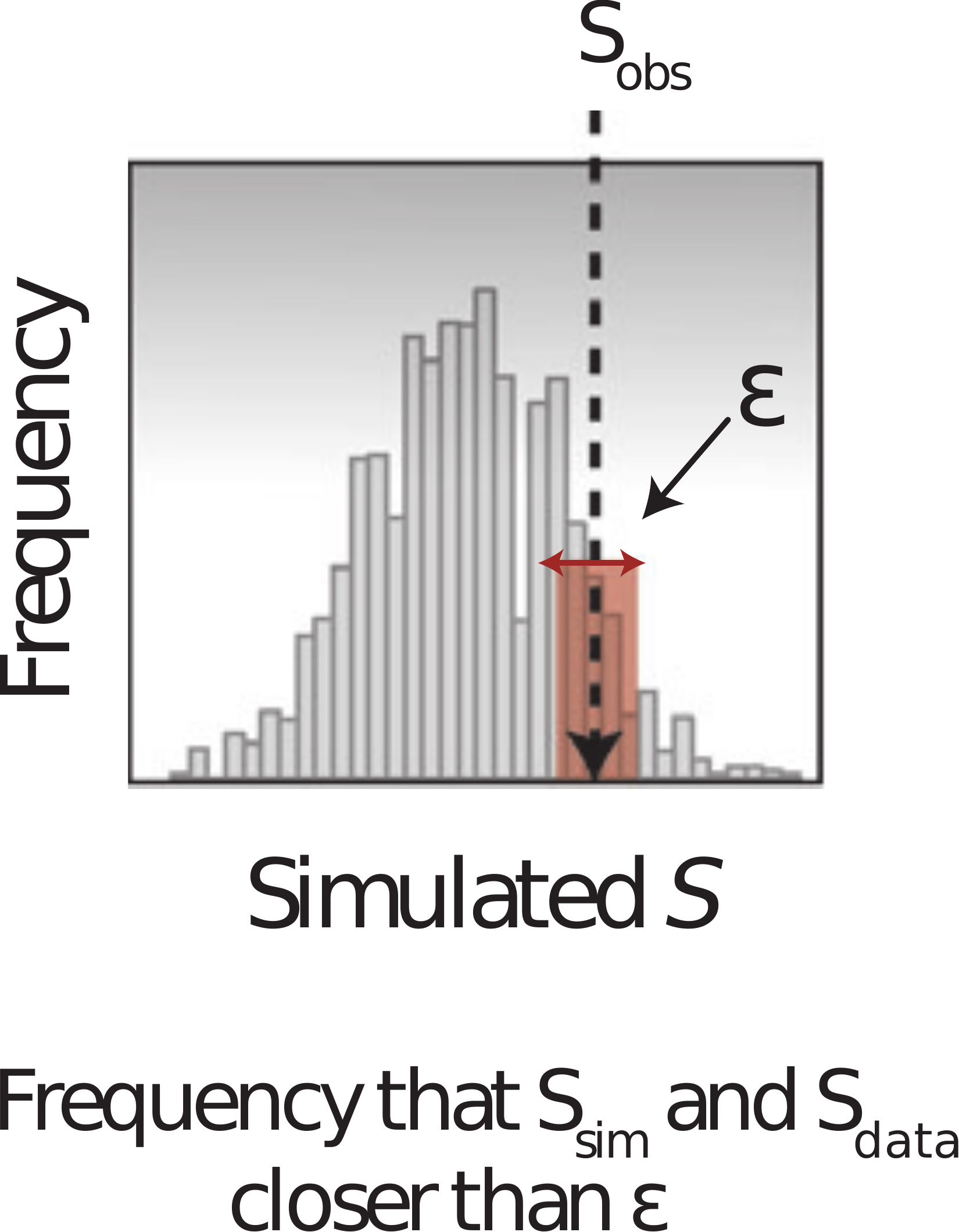
ABC approximates the likelihood using a set of summary statistics \(S\).
A summary statistic is
- something that is easy to calculate and approximates the likelihood
- e.g. final size, number of peaks, height or timing of peaks
The idea of sufficient summary statistics: to be exact, we would need summary statistics that give the same result as the likelihood.
The approximation
\[p(\text{data} \mid \theta) \approx p\big(d(S_\text{data},\, S_{\text{sim}(\theta)}) < \epsilon\big)\]
- \(S\): summary statistics
- \(d\): distance, e.g. absolute distance
- \(\epsilon\): acceptance window
Rejection ABC
The simplest version, and the one you will write:
- Sample \(\theta^*\) from the prior
- Simulate a dataset from the model at \(\theta^*\)
- Compute the distance \(d\) between simulation and data
- Keep \(\theta^*\) if \(d < \epsilon\), otherwise discard it
Repeat until you have enough. The kept parameters approximate the posterior.
No likelihood anywhere. Just a simulator, a distance, and a threshold.
Everything hangs on \(\epsilon\)
Too tight and you reject almost everything. The acceptance rate collapses and you wait forever for a handful of samples.
Too loose and you accept almost everything, including parameters that fit badly. In the limit you are sampling the prior.
There is no free lunch here: \(\epsilon\) trades accuracy against compute, and you cannot tell from inside the algorithm whether you have chosen well.
ABC-SMC
Rejection ABC wastes its effort: every draw comes from the prior, however hopeless.
ABC-SMC walks the threshold down in stages instead.
- Run rejection ABC at a loose \(\epsilon_1\)
- Perturb the accepted particles to propose for the next round
- Tighten to \(\epsilon_2 < \epsilon_1\) and repeat
Each generation starts from parameters already known to be reasonable, so far fewer simulations are wasted. Reaching a tight threshold becomes feasible.
The catch: particles need weighting to stay unbiased, which is the same propagate-weight-resample structure as the particle filter.
Is there a correct observation model?
No. There is only a choice, and the choice is part of the model.
- A likelihood is a distance function you have committed to in advance, with the benefit that it comes with a probabilistic interpretation.
- An ABC distance is a distance function you have chosen explicitly, with the benefit that it works when the likelihood is intractable.
Either way, be explicit about the choice and check whether your conclusions survive a different one.
Your Turn
In the practical you will
- fit the Tristan da Cunha data with Poisson and negative binomial observation models and compare
- see the likelihood plotted explicitly as a distance function
- implement ABC rejection sampling and ABC-SMC from scratch
- compare the posteriors, and test how each approach responds to an outlier
Observation models and ABC