MCMC diagnostics

Model fitting and inference for infectious disease dynamics

Recap

Review

In the practical you used Metropolis-Hastings with a Gaussian proposal distribution to infer a single parameter, \(R_0\).

In this session we will

  • extend to multivariate inference
  • learn about MCMC diagnostics
  • think about accuracy and efficiency

Interlude: the multivariate Gaussian

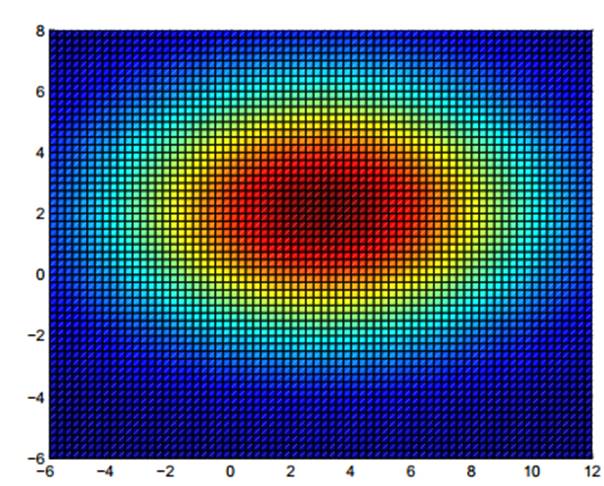
To infer several parameters at once we can use a multivariate Gaussian.

\(\mu = \begin{bmatrix} 3 & 2 \end{bmatrix}\), \(\Sigma = \begin{bmatrix} 25 & 0 \\ 0 & 9 \end{bmatrix}\)
\(\mu = \begin{bmatrix} 3 & 2 \end{bmatrix}\), \(\Sigma = \begin{bmatrix} 10 & 5 \\ 5 & 5 \end{bmatrix}\)
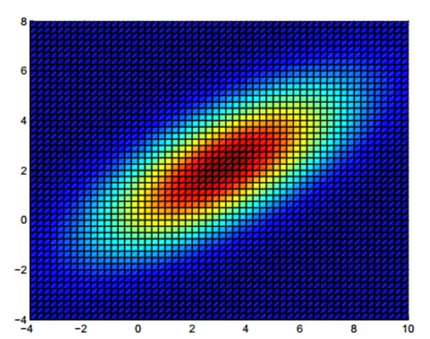
For accurate and efficient MCMC we tune the variance and the covariance of the proposal distribution.

Visual diagnostics

Why we like hairy caterpillars

Key characteristics:

  • Straight
  • Plump head, plump rear
  • Multiple colours

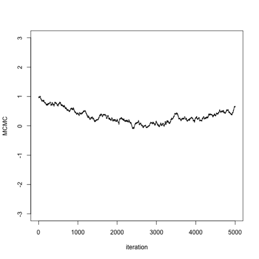
Choosing a proposal: too small

If the variance is too small, the chain will be slow to reach the target distribution.
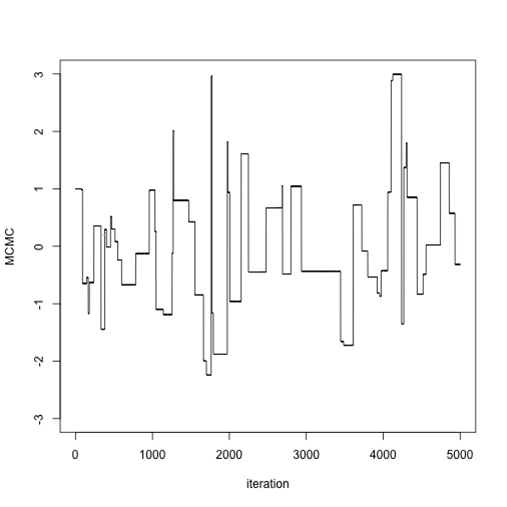
Choosing a proposal: too large

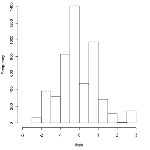
If the variance is too high, many proposed values will be rejected and the chain will stick in one place for many steps.
Choosing a proposal: about right

If the variance is just right, the chain efficiently explores the full shape of the target distribution.
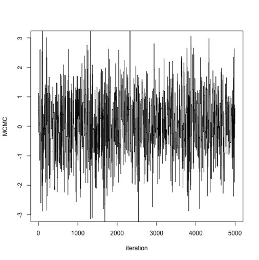
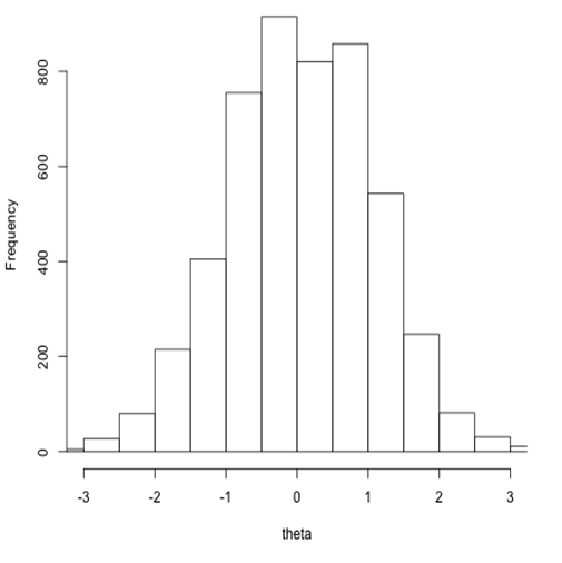
Try several proposal distributions (pilot runs), aiming for an acceptance rate between 24% and 40%.

Two more plots worth making

Running mean — the posterior mean recomputed as the chain grows.

It should settle and stay settled. Still drifting after thousands of iterations means the chain has not forgotten where it started, or has not finished exploring.

Autocorrelation — how correlated a sample is with the one \(k\) steps back.

It should decay towards zero within a few tens of lags. Still high at lag 100 means successive samples carry almost no new information, and your effective sample size is a small fraction of the iterations you ran.

Burn-in

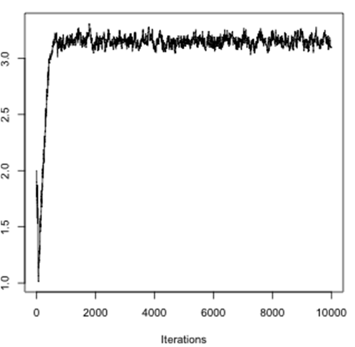
  • We can start our MCMC chain anywhere.

  • It can take a while to reach and explore the target density \(f(\theta)\).

  • Throw away the early samples: the burn-in phase.

  • How much to discard?

MCMC sample size

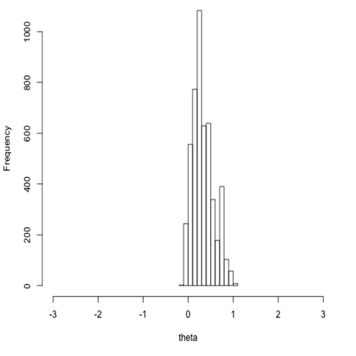
  • In MCMC each sample depends on the one before: auto-correlation.

  • Reduce auto-correlation by thinning, retaining only every \(n\)-th sample.

  • The information content of a set of MCMC samples is given by the effective sample size (ESS).

Accuracy and efficiency

How does each of these influence accuracy and efficiency?

  • Burn-in
  • MCMC iterations after burn-in
  • Thinning
  • Number of chains, with different initial conditions
  • Proposal distribution
  • Transforming parameters

Quantitative diagnostics

Running several chains

A single chain can look perfectly healthy and still be stuck in the wrong place.

Run several chains from different starting points. If they agree, that is evidence they have found the same distribution. If they disagree, at least one of them is wrong.

Four chains is a reasonable default.

R̂: the Gelman-Rubin diagnostic

Compare the variance within each chain to the variance between chains.

\[\hat{R} \approx \sqrt{\frac{\text{between-chain} + \text{within-chain}}{\text{within-chain}}}\]

  • If the chains have converged to the same distribution, \(\hat{R} \to 1\).
  • Chains sitting in different places inflate the between-chain variance and push \(\hat{R}\) up.

Rule of thumb: \(\hat{R} < 1.01\). Anything above 1.1 is a red flag.

Modern rank-normalised R̂ and ESS: Vehtari et al. (2021).

Effective sample size

MCMC samples are correlated, so \(N\) samples are worth fewer than \(N\) independent draws.

ESS estimates how many independent draws your chain is equivalent to.

  • ESS close to \(N\): efficient sampling, little autocorrelation
  • ESS far below \(N\): highly correlated, run longer
  • ESS below 100: not enough for reliable inference

Bulk ESS describes the centre of the distribution; tail ESS describes the extremes, and matters if you care about credible interval endpoints.

Monte Carlo standard error

ESS tells you how much information you have. MCSE turns that into the uncertainty on your estimate:

\[\text{MCSE} \approx \frac{\text{posterior SD}}{\sqrt{\text{ESS}}}\]

If the MCSE on your posterior mean is large relative to the effect you are reporting, you have not sampled enough — regardless of what the trace plot looks like.

Common failure modes

Divergent transitions

Specific to HMC and NUTS. The sampler simulates a trajectory; a divergence means that simulation became numerically unstable and flew off.

This usually means the posterior has a region of sharp curvature — a funnel or a narrow ridge — where the step size that works elsewhere is far too large.

A handful of divergences may be tolerable. Many means the sampler is systematically avoiding part of the posterior, so your samples are biased, not merely noisy.

Multimodality

If the posterior has several separated modes, a chain can settle in one and never see the others.

Multiple chains from different starting points are the standard detection: if they land in different modes, R̂ will be large.

Fixes are harder than detection. Reparameterisation sometimes helps; otherwise you need samplers designed to cross between modes.

A checklist

  1. Run at least four chains
  2. Look at the trace plots
  3. Check R̂ and ESS
  4. Check for divergences, if using NUTS
  5. Run a posterior predictive check — next session
  6. Rerun with more samples or a revised model if any of these fail

Your Turn

In the practical you will

  • generate good and bad chains and compare their trace plots
  • compute R̂, ESS and MCSE with MCMCChains
  • diagnose a deliberately badly specified model and try to fix it

References

Vehtari, Aki, Andrew Gelman, Daniel Simpson, Bob Carpenter, and Paul-Christian Bürkner. 2021. “Rank-Normalization, Folding, and Localization: An Improved for Assessing Convergence of MCMC.” Bayesian Analysis 16 (2): 667–718. https://doi.org/10.1214/20-BA1221.

Return to the session