Introduction to Markov Chain Monte Carlo
Model fitting and inference for infectious disease dynamics
Monte Carlo sampling
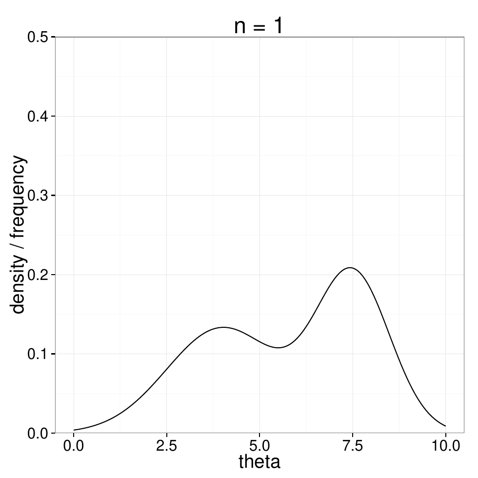
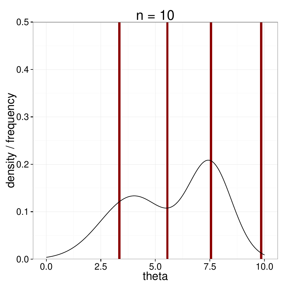
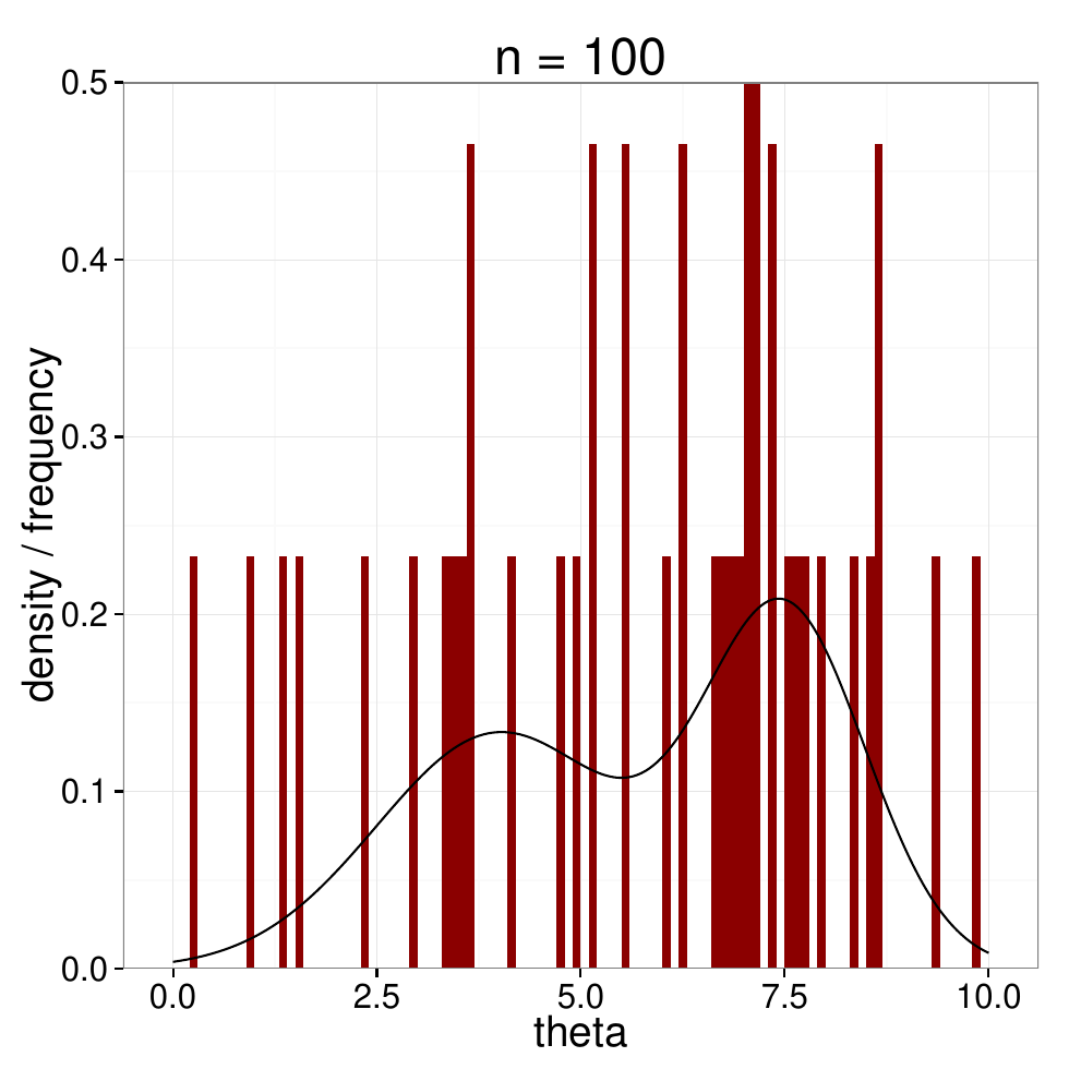
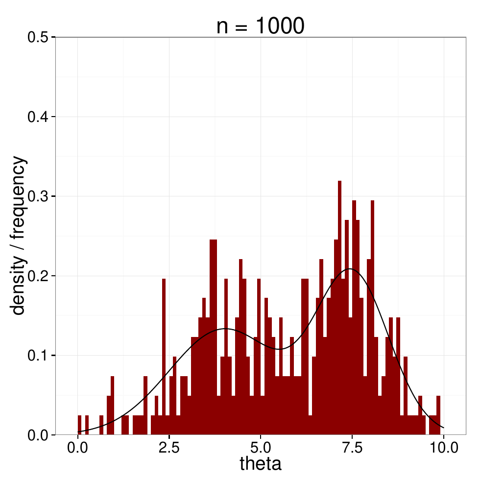
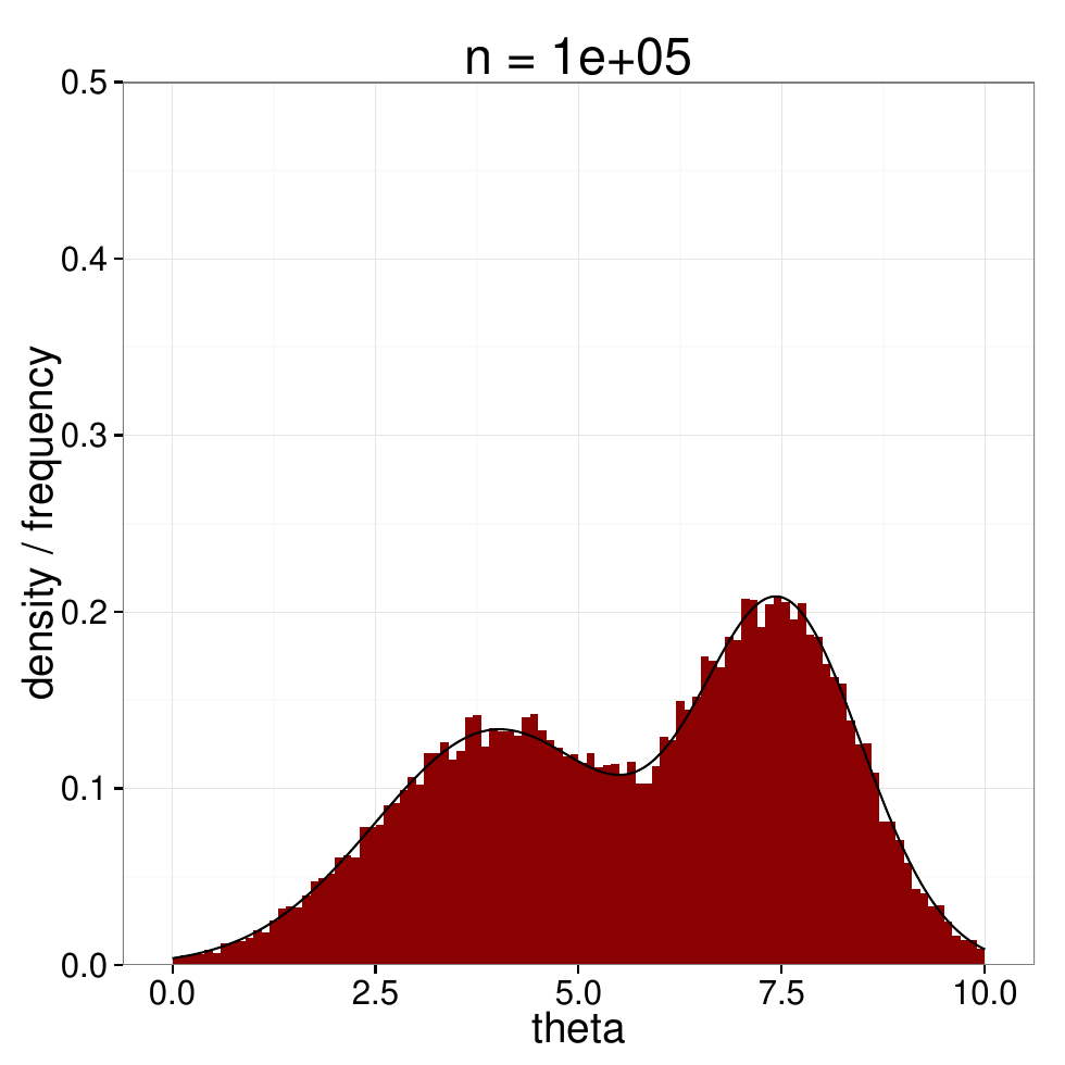
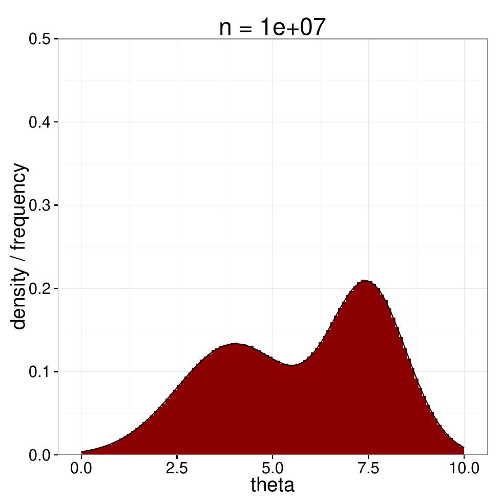
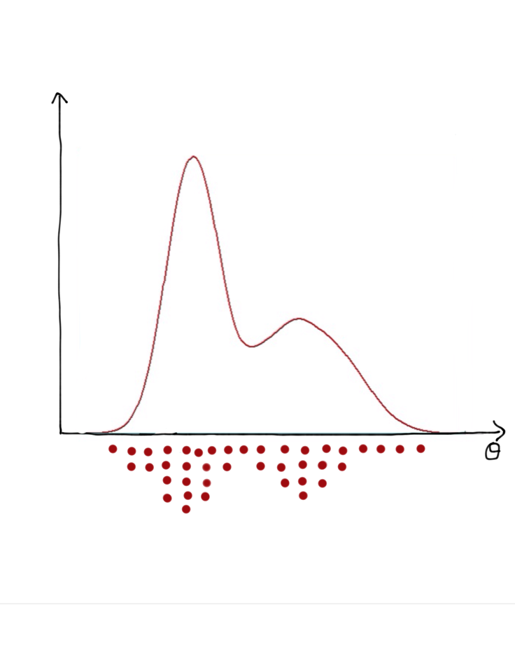
Explore a distribution by drawing from it. More samples, better picture:
Wasting time in sampling
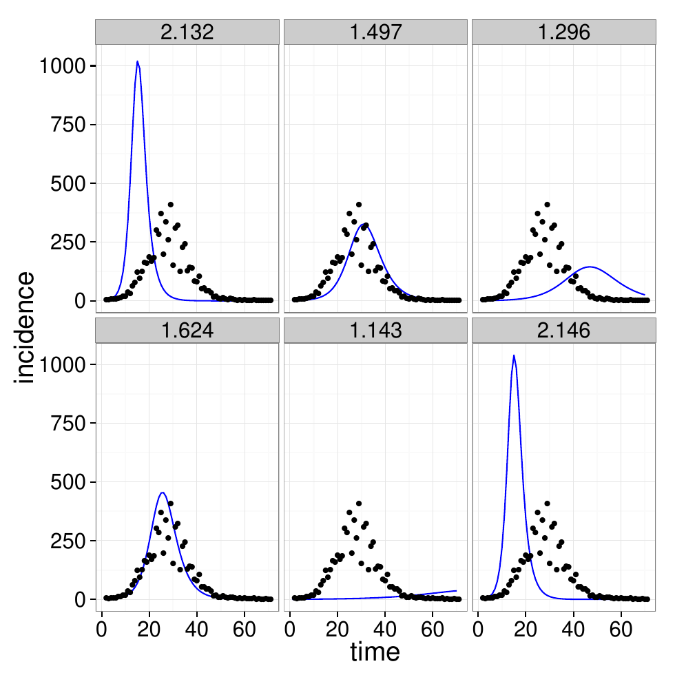
Sampling blindly from the prior spends almost all its effort on parameter values that fit the data badly. We need something that concentrates where the posterior is.
The problem
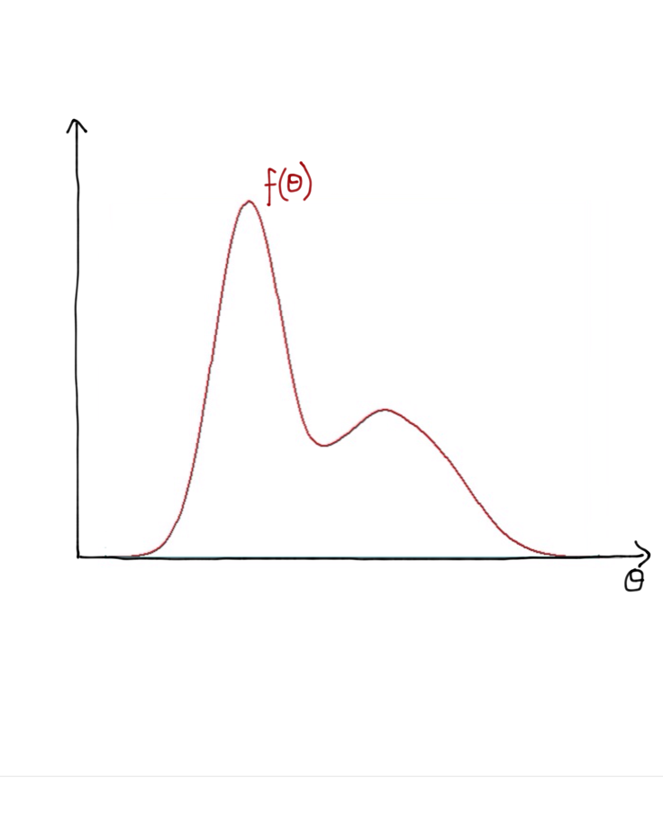
- Consider a distribution \(f(\theta)\) which we can evaluate for any \(\theta\)
- How do we draw samples from it?
A proposal distribution
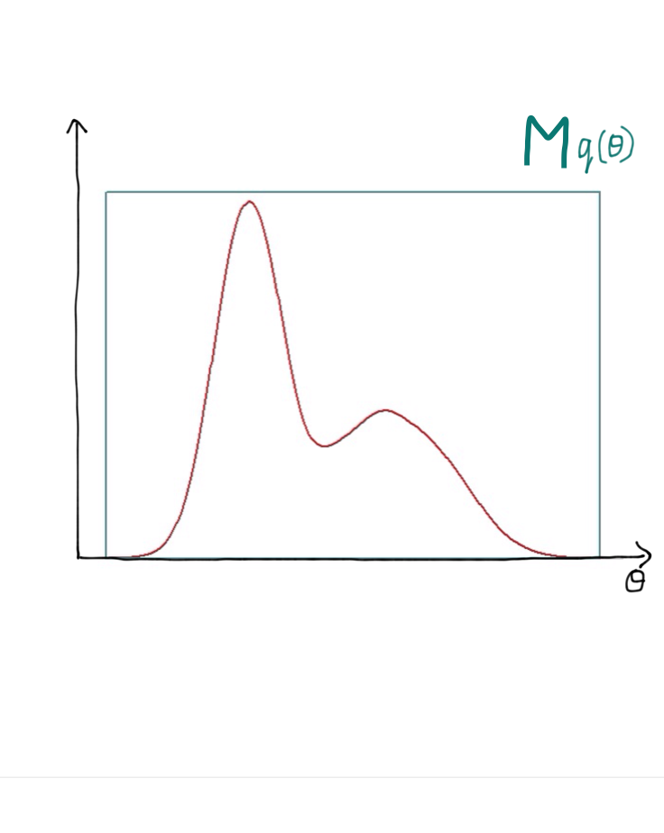
Rejection sampling uses a proposal distribution \(q(\theta)\) which
- is simple to evaluate
- is easy to sample from
- admits some \(M > 1\) with \(f(\theta) < M q(\theta)\) for all \(\theta\)
The algorithm
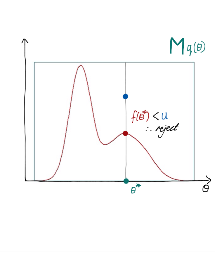
- Sample \(\theta^*\) from \(q(\theta)\)
- Draw \(u \sim \text{Uniform}[0,\, M q(\theta^*)]\)
- Evaluate \(f(\theta^*)\)
- If \(f(\theta^*) > u\) accept, else reject
- Repeat steps 1–4
Building up a sample
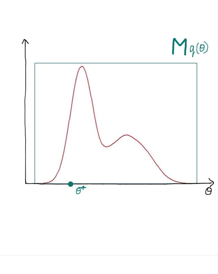
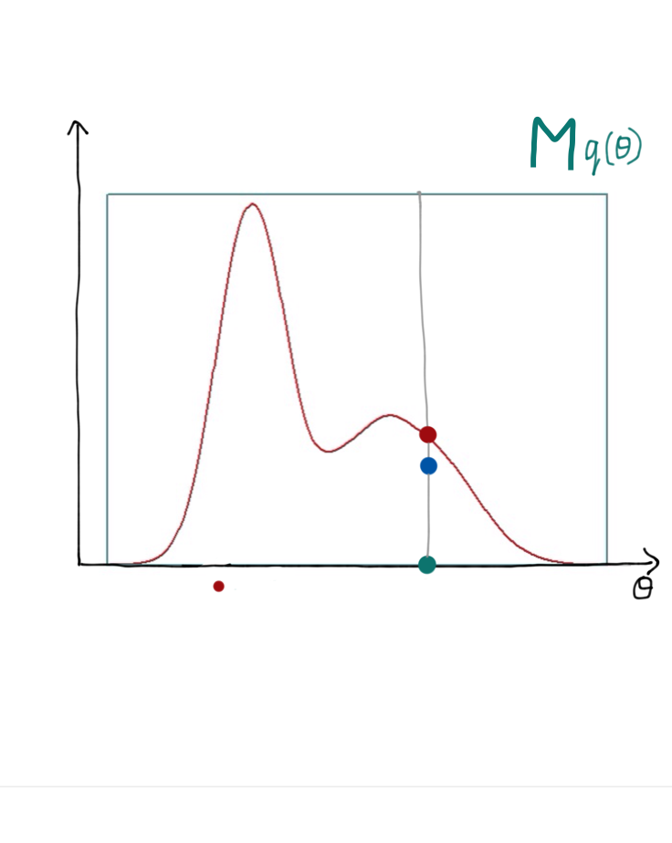
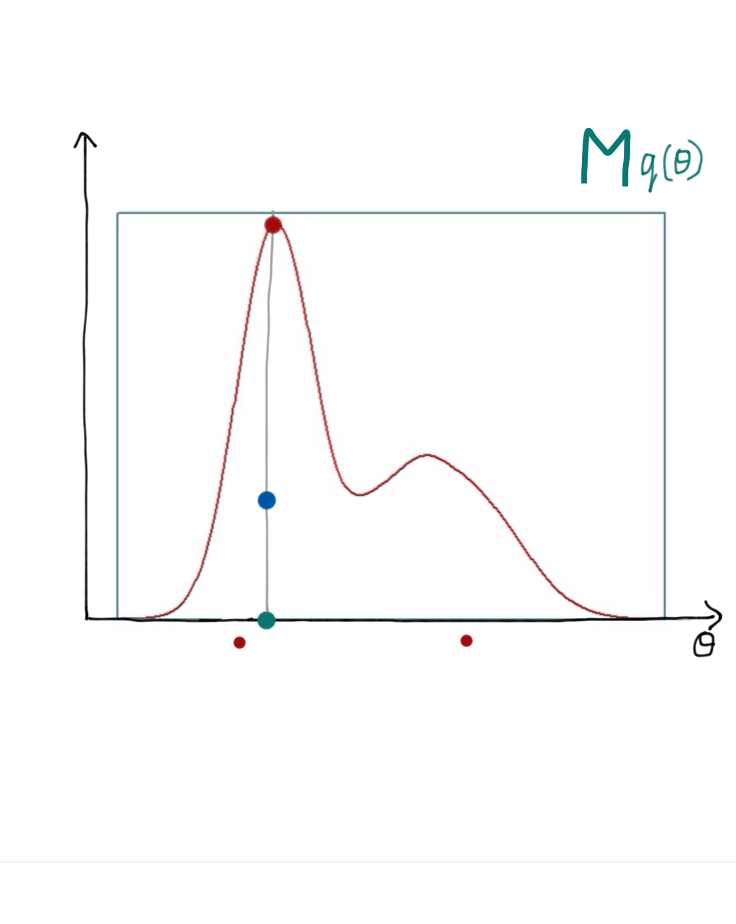
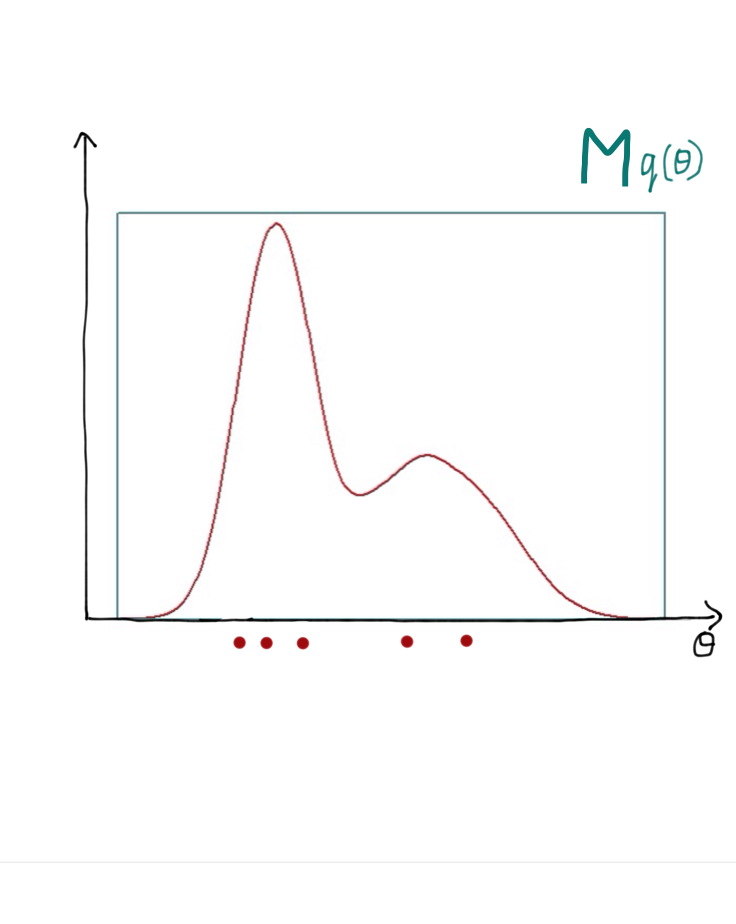
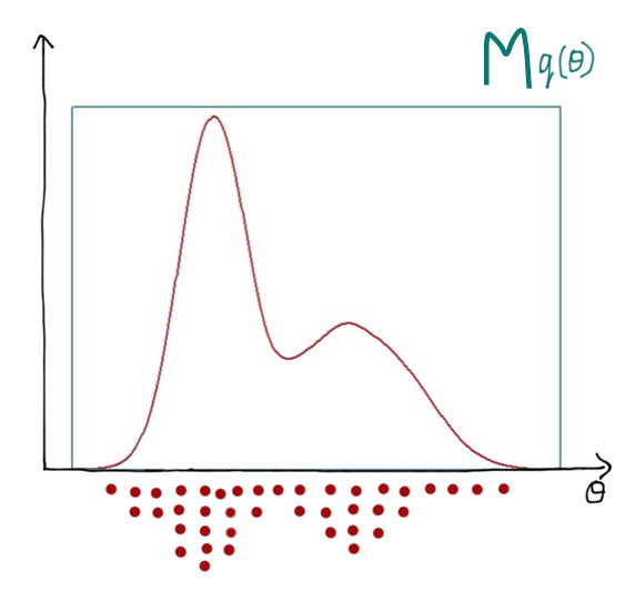
- Sample \(\theta^*\) from \(q(\theta)\)
- Draw \(u \sim \text{Uniform}[0,\, M q(\theta^*)]\)
- Evaluate \(f(\theta^*)\)
- If \(f(\theta^*) > u\) accept, else reject
- Repeat steps 1–4
Accepted points build up a sample from \(f(\theta)\).
When rejection sampling struggles
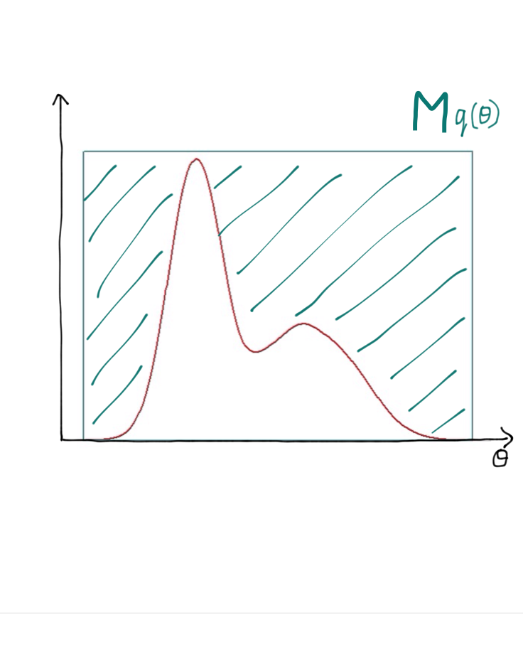
- Works best when \(q(\theta) \approx f(\theta)\), i.e. \(M \gtrapprox 1\)
- The acceptance rate is \(1/M\)
- Requiring \(f(\theta) < M q(\theta)\) everywhere can push the rejection rate very high
- Worse still in high dimensions
Metropolis-Hastings
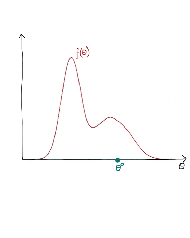
- Initialise \(\theta^{0}\), set \(\theta = \theta^{0}\)
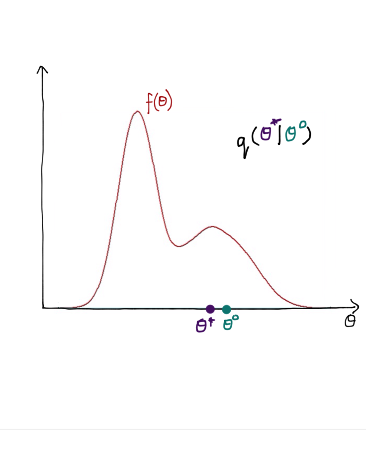
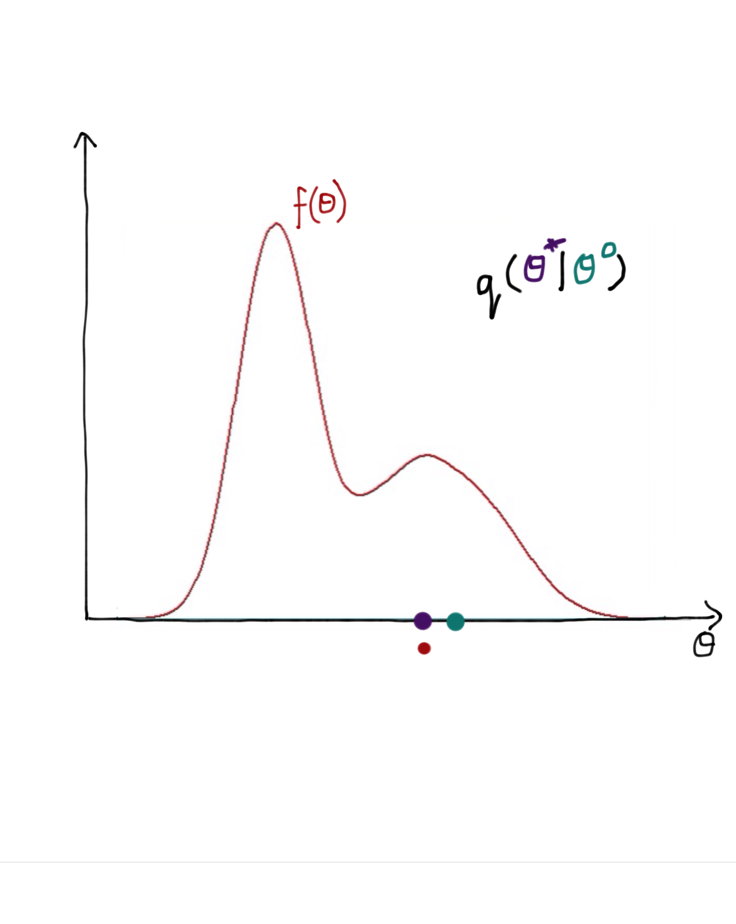
- Sample \(\theta^* \sim q(\theta^* \mid \theta)\)
- Compute the acceptance probability \(r\)
- Draw \(u \sim \text{Uniform}[0,1]\)
- Set the new sample to \[\theta^{(s+1)} = \begin{cases} \theta^*, & u < r\\ \theta^{(s)}, & u \geqslant r\end{cases}\]
- Repeat steps 2–5
The acceptance probability
If \(q(\theta^* \mid \theta)\) is symmetric, then
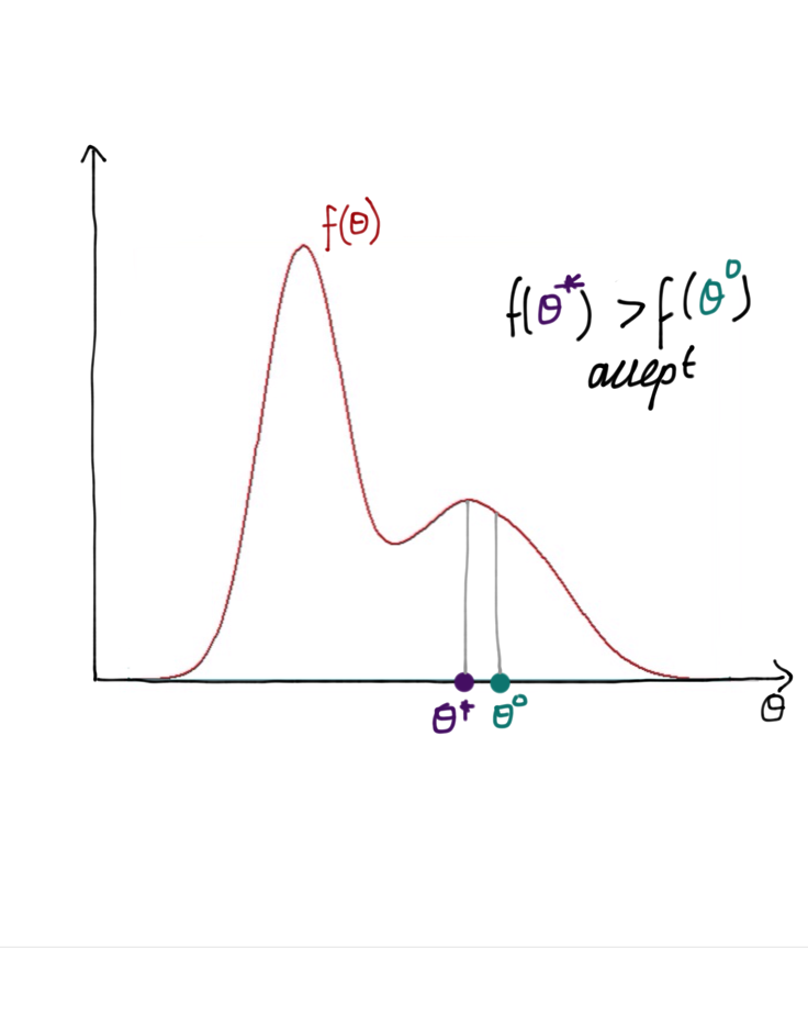
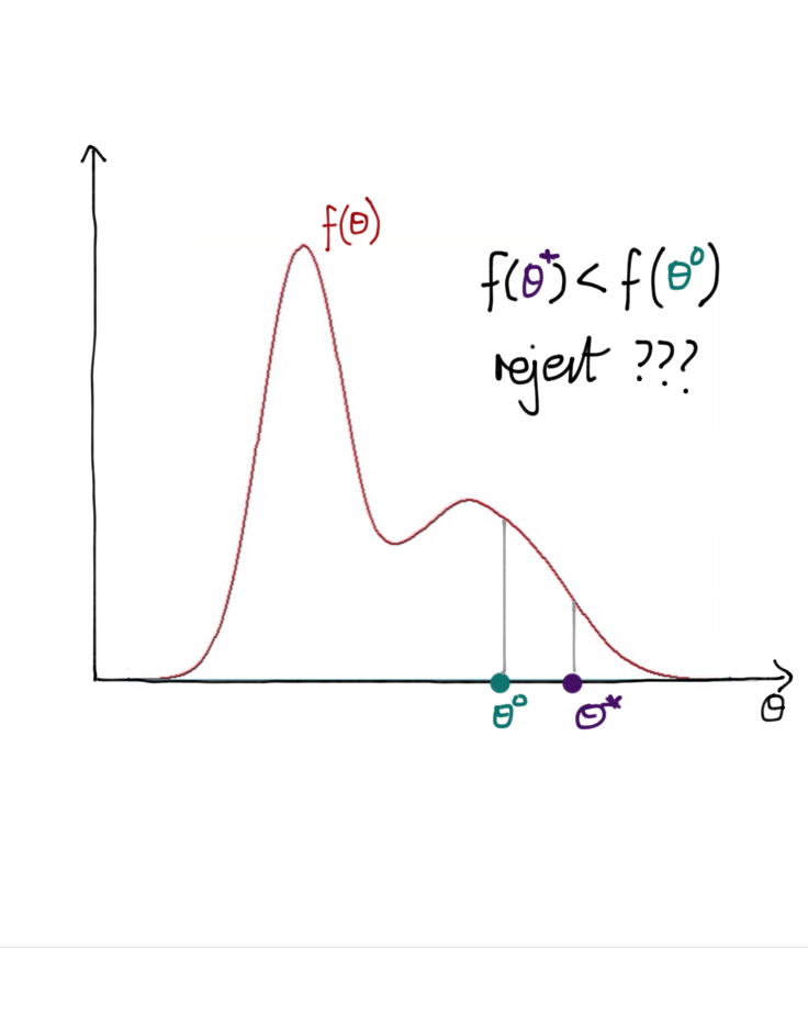
\[r = \min\left(1, \frac{f(\theta^*)}{f(\theta)}\right)\]
- Always move to \(\theta^*\) if it is more probable than \(\theta\)
- May move even if \(\theta^*\) is less probable
If \(q(\theta^* \mid \theta)\) is asymmetric, then
\[r = \min\left(1, \frac{f(\theta^*)\,q(\theta \mid \theta^*)}{f(\theta)\,q(\theta^* \mid \theta)}\right)\]
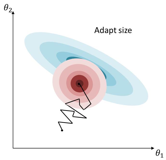
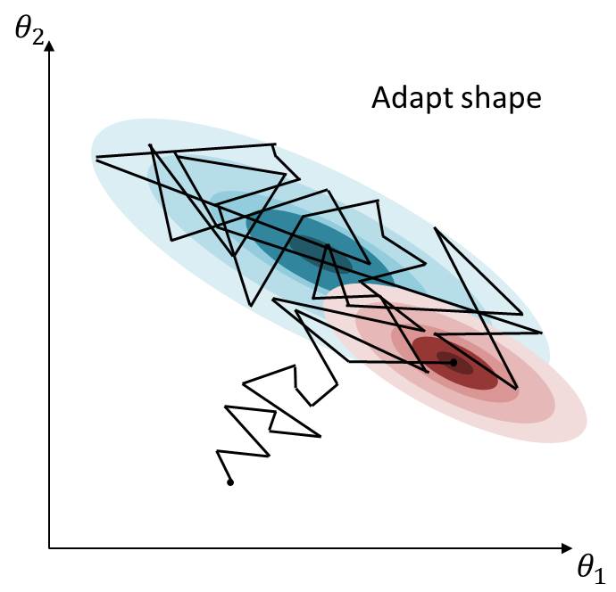
Adaptive MCMC: two-stage adaptation